KAPDEC® | Elite STEM Learning Platform | https://kapdec.com
Unit: Differential Equation
Chapter: Separable Differential Equation
Reference: – Reference: – Continuous, Discontinuous, Point of Discontinuity, Removable Discontinuity, jump discontinuity, Tangent line, Differentiation, Derivatives, Cusp, Critical point, Piecewise function, Continuity implication, Types of continuity & Differentiability, Mixed properties, Rules & Formation.
After studying this chapter, you should be able to:
- Separation of Variables & Integration technique.
- General, Existence & Uniqueness of solution.
- Particular Solution & Applications.
Introduction & Order of Equation

Source: Kapdec.com
(Differential Equation)
Basic Concepts
A differential equation is an equation that contains one or more terms that involve the derivatives of one variable (i.e., dependent variable) for the other variable (i.e., independent variable)
dy/dx = f(x)
Here “x” is an independent variable and “y” is a dependent variable
For example, dy/dx = 5x
The derivatives represent a rate of change, and the differential equation describes a relationship between the quantity that is continuously varying and the speed of change.
Order of a differential equation
The order of the differential equation is the order of the highest-order derivative present in the equation.
For example:
dy/dx = 3x + 2, the order is 1
Source: Kapdec.com
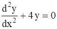
, the order is 2
Source: Kapdec.com
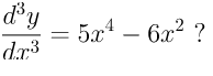
= 0, the order is 3
Example:
What is the order of the differential equation
dy/dx + 3x2 =4y?
Solution:
The order is the highest derivative, which in this case is 1.
Example:
What is the order of the differential equation
Solution:
Source: Kapdec.com
Solution:
The order is the highest derivative, which in this case is 3.
Degree of a differential equation
The degree of the differential equation is the order of the highest order derivative, where the original equation is represented in the form of a polynomial equation in derivatives such as y’, y”, y”’, and so on.
For example:
dy/dx + 1 = 0, the degree is 1
y”’ + 3y” + 6y’ – 12 = 0, degree is 1
Source: Kapdec.com
= 0, it is not a polynomial equation in y’, and the degree of such a differential equation can’t be defined.
Note: Order and degree (if defined) of a differential equation are always positive integers.
Example:
Determine the order and degree of each of the following differential equations. The state also whether they are linear or non-linear.
Source: Kapdec.com
Solution:
The order is the highest numbered derivative in the equation with no negative or fractional power of the dependent variable and its derivatives, while the degree is the highest power to which a derivative is raised.
So, in this question, the order of the differential equation is 2, and the degree of the differential equation is 1.
Separation of Variable & Integration Technique:
- Separation of variables is a technique used to solve certain types of ordinary differential equations where the variables can be separated on different sides of the equation.
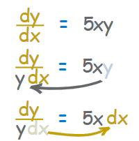
- The general form of a separable differential equation is dy/dx = f(x)g(y), where f(x) is a function of x and g(y) is a function of y.
- The goal of the separation of variables is to rearrange the equation so that all terms involving y are on one side and all terms involving x are on the other side.
- To separate the variables, one can divide both sides of the equation by g(y) and multiply both sides by dx. This allows the y terms to be isolated on one side and the x terms on the other side.
- After separating the variables, the resulting equation will typically be in the form g(y) dy = f(x) dx.
- Once the equation is in a separate form, you can integrate both sides of the equation for their respective variables. This involves integrating g(y) dy and f(x) dx separately.
- After integrating, you obtain an equation in form F(y) = G(x) + C, where F(y) and G(x) are the antiderivatives of g(y) and f(x), respectively, and C is the constant of integration.
- The equation F(y) = G(x) + C represents the general solution to the separable differential equation.
Source: Kapdec.com
(Variable separable equation)
Integration Techniques & Solution: –
- Integration of g(y) dy: Integrate the left side of the separated equation, which involves finding the antiderivative of the function g(y) for y.
- Integration of f(x) dx: Integrate the right side of the separated equation, which involves finding the antiderivative of the function f(x) for x.
- The constant of integration: After integrating both sides, you will obtain an equation of form F(y) = G(x) + C, where F(y) and G(x) are the antiderivatives of g(y) and f(x), respectively, and C is the constant of integration.
- Evaluate the constant of integration: If initial conditions are provided, you can use them to determine the value of the constant of integration (C).
- Simplification and additional steps: After evaluating the constant of integration, you may need to simplify the equation or perform additional algebraic manipulations to express the solution in a more suitable form.
- Check for validity: Finally, it is important to check the validity of the obtained solution by differentiating it and substituting it back into the original differential equation.
Particular Solution & Applications: –
- Applications: Separable differential equations find applications in various fields of mathematics and science. Some common applications include population dynamics, radioactive decay, chemical reactions, growth models, fluid flow, and electrical circuits.
- General Solution: When solving a separable differential equation, the goal is to find the general solution. The general solution represents a family of solutions that satisfy the differential equation. It contains a constant integration that allows for different specific solutions within the family.
- Initial Conditions: To obtain a specific solution from the general solution, we need to apply initial conditions. These conditions specify the value(s) of the dependent variable(s) at a particular point or time.
- Existence and Uniqueness: It is important to note that not all separable differential equations have unique solutions. The existence and uniqueness of solutions depend on certain conditions.
- Singular Solutions: In some cases, a separable differential equation may have singular solutions. These solutions arise when the constant of integration takes a particular value.
- Phase Diagrams: Separable differential equations can be represented graphically using phase diagrams. Phase diagrams illustrate the behavior of the solutions over time or for different initial conditions.
- Numerical Methods: In situations where analytical solutions are not readily obtainable, numerical methods such as Euler’s method, Runge-Kutta methods, or finite difference methods can be employed to approximate the solutions of separable differential equations.
Key Points
- Separable differential equations are a specific type of ordinary differential equation (ODE) that can be written in the form f(y) dy = g(x) dx.
- The term “separable” refers to the ability to separate the variables, isolating all terms involving y on one side and all terms involving x on the other side of the equation.
- The separation of variables allows for the solution of the differential equation by integrating both sides concerning their respective variables.
- The integration of the left side typically involves finding the antiderivative of the function f(y) for y.
- The integration of the right side typically involves finding the antiderivative of the function g(x) for x.
- After integration, a constant of integration is introduced to account for the family of solutions that satisfy the differential equation.
- The constant of integration can be determined by applying initial conditions or boundary conditions to find the particular solution.
- Separable differential equations have a wide range of applications in various fields, including physics, biology, economics, and engineering.
- They are particularly useful in modeling exponential growth or decay, population dynamics, and chemical reactions.
- Numerical methods can be used to approximate solutions for separable differential equations when analytical solutions are not readily obtainable.
