KAPDEC® | Elite STEM Learning Platform | https://kapdec.com
Unit: Graphing: Interpretation
Chapter: Rate of Change and Impact on Function Manipulation
Reference: – Concept of Rate of Change in Functions, Average Rate of Change Over an Interval, Instantaneous Rate of Change, Slope of Linear Functions as Constant Rate of Change, Interpreting Non-Linear Rate of Change, Effect of Changing Slope on the Graph, Vertical Stretch and Compression in Functions, Horizontal Stretch and Compression in Functions, Effect of Reflection over Axes, Vertical Shifts of Functions, Understanding Slope as Rate of Change in Context
After studying this chapter, you should be able to understand:
- Concept of Rate of Change in Functions & Average Rate of Change Over an Interval
- Instantaneous Rate of Change & Slope of Linear Functions as Constant Rate of Change
- Effect of Changing Slope on the Graph & Vertical Stretch and Compression in Functions
- Understanding Slope as Rate of Change in Context
- Concept of Rate of Change in Functions:
The rate of change describes how one quantity varies with respect to another in a function. It measures the relationship between the input (independent variable) and output (dependent variable) over an interval.
- Average Rate of Change Over an Interval:
This is the change in the output values divided by the change in input values over a specific interval. It represents the overall rate of change between two points on a graph.
- Instantaneous Rate of Change:
The instantaneous rate of change refers to how fast a function is changing at a particular point. It is conceptually linked to the slope of the tangent line at that specific point on the curve.
- Slope of Linear Functions as Constant Rate of Change:
For linear functions, the rate of change remains constant across all intervals. The slope is a measure of this constant rate of change and determines the angle of the graph with respect to the x-axis.
- Interpreting Non-Linear Rate of Change:
In non-linear functions, the rate of change varies at different points. The slope between any two points on the curve can change, indicating acceleration, deceleration, or variable growth.
- Effect of Changing Slope on the Graph:
Altering the slope in a linear function affects the steepness and direction of the graph. A larger absolute slope makes the graph steeper, while the sign of the slope determines if the function is increasing or decreasing.
- Vertical Stretch and Compression in Functions:
Multiplying a function’s output by a constant result in vertical stretching or compression. A stretch makes the graph taller (increased output values), while a compression makes it shorter (decreased output values).
- Horizontal Stretch and Compression in Functions:
Manipulating the input variable by multiplying it by a constant leads to horizontal stretching or compression. This changes how quickly the output grows with respect to input.
- Effect of Reflection over Axes:
Reflecting a function over the x-axis or y-axis changes the orientation of the graph. A reflection over the x-axis reverses the sign of the output values, while a reflection over the y-axis reverses the input values.
- Vertical Shifts of Functions:
Adding or subtracting a constant to the entire function shifts the graph upward or downward along the y-axis. This affects the vertical position but does not change the shape of the graph.
- Horizontal Shifts of Functions:
Changing the input variable by adding or subtracting a constant shifts the graph left or right along the x-axis. This alters where the function starts or peaks horizontally.
- Understanding Slope as Rate of Change in Context:
In real-world contexts, the slope or rate of change represents specific measurable rates, such as speed, price rate, growth, or decline per unit time or distance.
- Interpreting Rate of Change from Graph Shape:
By observing the graph’s shape (whether it curves upwards, downwards, or stays linear), one can infer whether the rate of change is increasing, decreasing, or constant.
- Comparing Rates of Change Between Different Functions:
This involves analysing multiple functions to determine which grows faster, declines more quickly, or remains more stable. Both visual inspection and algebraic comparison can help determine this.
- Predicting Future Values Based on Rate of Change:
By understanding the pattern and rate at which a function changes, future output values can be estimated or predicted based on current and past behavior.
Example: –
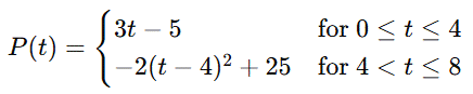
A company tracks its profit over time with the following piecewise function:
Source: Kapdec.com
Where:
- P(t) = Profit in thousands of dollars
- t = Time in years
Tasks:
- Calculate the average rate of change of profit from t=0 to t=8.
- Find the instantaneous rate of change at t=4 (from both sides, if needed).
- Identify and explain how function manipulation (stretch, shift, reflection) affects the graph between the two intervals.
Solution: –
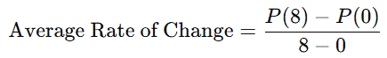
Average Rate of Change from t=0t to t=8:
Formula:
Source: Kapdec.com
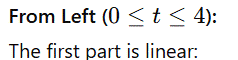
First find P(0):
From the first piece (linear):
Source: Kapdec.com
Next find P(8):
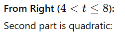
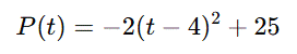
From the second piece (quadratic):
Source: Kapdec.com
Now calculate:
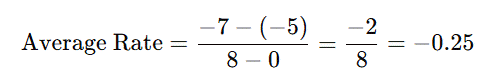
Source: Kapdec.com
The average rate of change from year 0 to year 8 is −0.25 thousand dollars per year, indicating an overall decrease in profit.
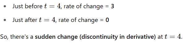
Instantaneous Rate of Change at t=4:
For piecewise functions, we calculate the slope from both sides (left-hand and right-hand limits):
Source: Kapdec.com
Source: Kapdec.com
Source: Kapdec.com
Source: Kapdec.com
Derivative of the second part (instantaneous rate of change):
Source: Kapdec.com
At t=4:
Source: Kapdec.com
Source: Kapdec.com
Graph Transformations (Function Manipulation Impact):
Between the two intervals:
- First Interval (Linear Function):
Original linear function with slope 3, shifted down by 5 units (vertical shift). - Second Interval (Quadratic Function):
A downward-opening parabola (due to the negative coefficient),
horizontally shifted right by 4 units,
and vertically shifted up by 25 units,
with a vertical stretch by a factor of 2 (due to the -2 multiplier).
Final Interpretation:
- From years 0 to 4: Steady linear growth in profit.
- At year 4: A sudden change in trend, from rising profit to a peak followed by a sharp decrease (parabolic fall).
- From 4 to 8 years: Decreasing profit at a non-constant rate.
Here are five conclusive points for “Linear Functions in a Coordinate Plane”:
- Understanding Rate of Change Helps Predict Behavior:
Analysing how one variable changes with respect to another allows students to predict future trends, identify growth patterns, and model real-world scenarios effectively.
- Slope Provides Critical Insight into Function Dynamics:
In both linear and non-linear functions, the slope or rate of change gives immediate visual and mathematical information about the direction, speed, and consistency of change.
- Graph Manipulations Directly Affect Function Behavior:
Transformations like shifts, stretches, compressions, and reflections change the appearance of the graph and the relationship between input and output values, allowing for customized modeling.
- Real-World Applications Depend on Rate Interpretation:
In fields like physics, economics, biology, and engineering, understanding and manipulating the rate of change in functions is crucial for solving real-life problems such as speed, cost, population dynamics, and resource consumption.
- Visual Representations Enhance Conceptual Understanding:
Graphing functions and observing their transformations help students make deeper connections between algebraic equations and their geometric interpretations, improving problem-solving and analysis skills.
Scan to visit this resource online
https://kapdec.com/resources/rate-of-change-and-impact-on-function-manipulation
