KAPDEC® | Elite STEM Learning Platform | https://kapdec.com
Unit: Exploring Two – Variable Data
Chapter: Associations & Interpreting Correlations
Reference: – Correlation coefficient, Scatter plots, Causation vs correlation, Pearson correlation coefficient, Spearman rank correlation, Kendall’s Tau, Coefficient of determination, Confounding variables, Outliers, strength of correlation.
After studying this chapter, you should be able to understand:
- Correlation coefficient & Scatter plots.
- Causation vs correlation & Pearson correlation coefficient.
- Spearman Rank correlation & Kendall’s Tau.
- Coefficient of determination & Confounding variables
Correlation Coefficient & Scatter plots
Correlation Coefficient:
- The correlation coefficient (r) measures the strength and direction of a linear relationship between two quantitative variables.
- The value of r ranges between -1 and +1. A positive value indicates a positive correlation (both variables tend to increase together), while a negative value indicates a negative correlation (one variable tends to decrease as the other increases).
- An r value closer to 1 or -1 indicates a stronger linear relationship, while an r value closer to 0 suggests a weaker relationship.
- The sign of r (positive or negative) indicates the direction of the linear relationship, while the magnitude (absolute value) indicates the strength.
- Correlation does not imply causation. Even a strong correlation does not prove that changes in one variable cause changes in the other.
- The formula for calculating the correlation coefficient is sensitive to the units of measurement, but it is unitless.
- Outliers can significantly affect the value of r, potentially inflating or diminishing the correlation.
- The Pearson correlation coefficient assumes linearity and normal distribution of data. It may not be appropriate for non-linear relationships or skewed data.
- A correlation of 0 does not necessarily mean there’s no relationship between the variables; it indicates that there’s no linear relationship.
Scatter Plots:
- Scatter plots are graphical representations of paired data points, with one variable plotted on the x-axis and the other on the y-axis.
- Scatter plots help visualize the relationship between two variables and identify patterns, trends, or clusters.
- The pattern of points on a scatter plot can suggest the type of relationship between the variables: linear, exponential, quadratic, etc.
- When interpreting a scatter plot, look for the overall direction of the points (upward, downward, or no clear pattern) and the spread or concentration of points.
- A linear relationship between variables is often indicated by points forming a roughly straight line on the scatter plot.
- Scatter plots can reveal outliers, which are data points that significantly differ from the rest of the data and can impact the interpretation of the relationship.
- The line of best fit (regression line) is a straight line that best represents the general trend of the data points on a scatter plot.
- The line of best fit minimizes the sum of the squared vertical distances (residuals) between the data points and the line.
- The correlation coefficient (r) is related to the slope of the line of best fit. The steeper the slope, the stronger the correlation.
- Scatter plots can help identify influential points, which have a significant impact on the slope and position of the regression line.
Causation vs correlation & Pearson correlation coefficient
Causation vs. Correlation:
- Causation: Causation implies a cause-and-effect relationship between two variables, where changes in one variable directly lead to changes in the other. Establishing causation often requires experimental design and controlling for confounding variables.
- Correlation: Correlation indicates a statistical association between two variables, but it does not necessarily imply a cause-and-effect relationship. Just because two variables are correlated does not mean that changes in one cause changes in the other.
- Common-Cause Fallacy: Assuming that because two variables are correlated, one must cause the other. However, a third variable (confounder) could be influencing both variables, leading to the correlation.
- Reverse Causation: Assuming that one variable cause another, when in reality, the direction of causation is the opposite. Correlation alone cannot determine the direction of causation.
- Spurious Correlations: Correlations that arise due to coincidence or the influence of a third variable, without any causal relationship between the variables.
- Experimental Design: Establishing causation often requires conducting controlled experiments, where one variable is deliberately manipulated to observe its impact on another variable.
- Randomized Controlled Trials (RCTs): Gold standard in experimental design, where participants are randomly assigned to different groups to assess the causal effect of a treatment or intervention.
- Observational Studies: Correlations are often identified through observational studies, where researchers observe and collect data on variables without directly manipulating them.
Pearson Correlation Coefficient:
- The Pearson correlation coefficient (r) quantifies the strength and direction of a linear relationship between two continuous variables.
- The formula for calculating the Pearson correlation coefficient involves dividing the covariance of the variables by the product of their standard deviations.
- The value of r ranges from -1 to +1. A positive value indicates a positive linear relationship, a negative value indicates a negative linear relationship, and 0 indicates no linear relationship.
- The magnitude of r indicates the strength of the correlation. Values closer to 1 or -1 indicate a stronger correlation, while values closer to 0 suggest a weaker correlation.
- The Pearson correlation coefficient assumes linearity and normal distribution of data. It may not accurately capture non-linear relationships.
- Correlation does not imply causation. Even a strong correlation does not prove that changes in one variable cause changes in the other.
- The Pearson correlation coefficient is sensitive to outliers, which can distort the calculated correlation.
- The coefficient only measures the strength and direction of linear relationships; it may not capture other types of associations.
- It is important to consider the context and subject matter expertise when interpreting correlation coefficients.
- Scatter plots are often used to visualize the relationship between variables and help interpret the Pearson correlation coefficient.
- Causation requires additional evidence beyond correlation, such as experimental design or a strong theoretical framework.
- A correlation coefficient of 0 does not necessarily imply no relationship between variables; it indicates no linear relationship specifically.
- Interpreting a correlation coefficient involves understanding both its sign (positive/negative) and its magnitude.
- In some cases, a low correlation coefficient might be misleading, as it could result from the presence of confounding variables or a non-linear relationship.
- When interpreting correlation, consider its limitations and potential sources of bias or error in the data collection process.
Spearman Rank correlation & Kendall’s Tau
Spearman Rank Correlation:
- The Spearman rank correlation (ρ or “rho”) measures the strength and direction of a monotonic relationship between two variables.
- Monotonicity implies that as one variable increases, the other variable tends to also increase or decrease, without requiring a linear relationship.
- Spearman’s rho is appropriate for variables that may have a non-linear or non-normally distributed relationship.
- In situations where the data is not quantitative or the relationship is not clearly linear, Spearman rank correlation provides a useful alternative to Pearson correlation.
- The Spearman correlation is calculated by first assigning ranks to the data points for each variable, then calculating the Pearson correlation coefficient for the ranks.
- The value of ρ ranges from -1 to +1. A positive value indicates a positive monotonic relationship, while a negative value indicates a negative monotonic relationship.
- Just like Pearson correlation, Spearman rank correlation does not imply causation; it only quantifies the strength and direction of an association.
- Spearman rank correlation is less sensitive to outliers compared to Pearson correlation, since it focuses on the order or rank of the data points rather than their exact values.
- It can be particularly useful when dealing with ordinal data or when the variables have a qualitative or categorical nature.
Kendall’s Tau:
- Kendall’s Tau (τ) is another rank-based correlation coefficient that measures the strength and direction of association between two variables.
- Like Spearman rank correlation, Kendall’s Tau is appropriate for identifying monotonic relationships, regardless of whether the relationship is linear.
- Kendall’s Tau is calculated by comparing pairs of data points to see if they have the same order in both variables, and then using this information to compute a correlation coefficient.
- Kendall’s Tau is unaffected by tied ranks, where multiple data points have the same rank, making it robust for situations with tied data.
- The value of τ ranges from -1 to +1, similar to other correlation coefficients. Positive values indicate positive association, and negative values indicate negative association.
- Kendall’s Tau is often used when the sample size is small or when dealing with ranked or ordinal data.
- Kendall’s Tau is also less sensitive to outliers compared to Pearson correlation, making it suitable for data with potential outliers.
- Just like other correlation measures, Kendall’s Tau does not establish causation.
- Both Spearman rank correlation and Kendall’s Tau provide alternatives to Pearson correlation when the assumptions of linearity and normal distribution are not met.
- Interpreting Kendall’s Tau involves understanding the direction and strength of association based on the calculated coefficient.
- As with any statistical measure, it’s important to consider the context and potential limitations of Kendall’s Tau when interpreting results.
- Kendall’s Tau is commonly used in social sciences, economics, and other fields where the variables may not have a linear relationship.
- The choice between Spearman rank correlation and Kendall’s Tau may depend on the specific characteristics of the data and the research question.
- Both Kendall’s Tau and Spearman rank correlation provide valuable insights into the relationships between variables, especially when linear correlation may not be appropriate.
- Understanding the assumptions and appropriate applications of these rank-based correlation measures is essential for accurate data analysis and interpretation.
Coefficient of determination & Confounding variables
Coefficient of Determination (R-squared):
- The coefficient of determination (R-squared) is a statistical measure that represents the proportion of the variance in the dependent variable that is explained by the independent variable(s) in a linear regression model.
- R-squared values range from 0 to 1. A higher R-squared indicates that a larger proportion of the variability in the dependent variable is accounted for by the independent variable(s).
- R-squared can be interpreted as the goodness of fit of the regression model to the data. A value of 1 indicates a perfect fit, while a value of 0 indicates that the model does not explain any variability.
- R-squared is calculated as the ratio of the explained sum of squares (ESS) to the total sum of squares (TSS). Mathematically, R-squared = ESS / TSS.
- While a high R-squared suggests a strong relationship between variables, it does not indicate causation. A high R-squared could be due to a confounding variable or other factors not considered in the model.
- R-squared may lead to overfitting if additional variables are added to the model that do not have theoretical or practical relevance, resulting in a higher R-squared but a less interpretable and useful model.
- R-squared can be misleading if applied to models with nonlinear relationships, as it only quantifies the fit of a linear model.
- Adjusted R-squared takes into account the number of variables in the model and adjusts R-squared to penalize the inclusion of unnecessary variables. It helps prevent overfitting.
- R-squared should be interpreted within the context of the research question and subject matter expertise, as high R-squared values do not necessarily imply a meaningful or significant relationship.
Confounding Variables:
- Confounding variables are extraneous factors that are not included in a statistical analysis but can influence the relationship between the independent and dependent variables.
- Confounders can lead to incorrect conclusions about the true relationship between variables. They create a spurious association that may be mistakenly attributed to the variables of interest.
- Controlling for confounding variables is crucial to establish causal relationships. This can be achieved through experimental design, randomization, or statistical techniques like regression analysis.
- Confounding can arise in observational studies, where researchers cannot control the assignment of participants to different conditions.
- In experimental studies, random assignment helps minimize the impact of confounders by distributing their effects evenly across treatment groups.
- In regression analysis, controlling for confounders involves including them as independent variables in the model to isolate the effect of the variable of interest.
- Matching or stratification can be used to group subjects based on potential confounders, ensuring that each group has a similar distribution of those variables.
- Simpson’s Paradox is a phenomenon where a confounding variable leads to a reversal of the direction of an association when subgroups are analyzed separately from the overall data.
- Careful consideration of potential confounders and their inclusion in the analysis is essential for accurate and meaningful results.
- In some cases, it may be challenging to identify and control for all confounding variables, which highlights the importance of cautious interpretation and acknowledging potential limitations in the conclusions drawn from the analysis.
Example: Examining the Relationship Between Study Time and Test Scores
A teacher wants to investigate the relationship between the amount of time students spend studying for an exam and their corresponding test scores. The teacher collects data from a sample of 20 students and records their study hours and test scores. The goal is to determine if there is a correlation between study time and test scores and to interpret the strength and direction of the correlation.
Here is the dataset:
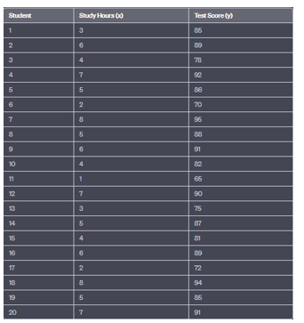
Source: Kapdec.com
Solution: – To examine the relationship between study time and test scores, we will calculate the Pearson correlation coefficient (r) and interpret its value.
Step 1: Calculate the Pearson Correlation Coefficient (r) To calculate r, we need to calculate several sums and products:
- Sum of study hours (Σx) = 100
- Sum of test scores (Σy) = 1734
- Sum of the product of study hours and test scores (Σxy) = 13855
- Sum of the squared study hours (Σx²) = 716
- Sum of the squared test scores (Σy²) = 153395
Using the formula for r:
r = (nΣxy – ΣxΣy) / √[(nΣx² – (Σx)²)(nΣy² – (Σy)²)]
Substituting the values:
r = (20 * 13855 – (100 * 1734)) / √[(20 * 716 – (100)²)(20 * 153395 – (1734)²)] r ≈ 0.876
Step 2: Interpret the Result The calculated Pearson correlation coefficient (r) is approximately 0.876.
Interpretation:
- The positive value of r (0.876) indicates a positive correlation between study time and test scores.
- The correlation is moderately strong, suggesting that as study time increases, test scores tend to increase as well.
- However, it’s important to note that correlation does not imply causation. While this correlation suggests a relationship between study time and test scores, other factors could be influencing test scores.
In conclusion, the analysis shows a moderate positive correlation between study time and test scores. Students who study more hours generally tend to achieve higher test scores. However, other variables not considered in this analysis could also impact test scores, so causation cannot be inferred solely from this correlation.
Scan to visit this resource online
https://kapdec.com/resources/associations-interpreting-correlations
