KAPDEC® | Elite STEM Learning Platform | https://kapdec.com
Unit: Exponential & Logarithmic Functions
Chapter: Growth Patterns: Sequences and Exponential Models
Reference: – Introduction to Sequences, Explicit and Recursive Formulas, Geometric Sequences in Depth, Exponential Growth Models, Exponential Decay Models, Compound Interest & Continuous Growth, Connection Between Geometric Sequences & Exponential Functions, Graphical Representation of Exponential Functions, Model Fitting with Data, Applications in Real-World Problems
After studying this chapter, you should be able to:
- Introduction to Sequences & Explicit and Recursive Formulas
- Connection Between Geometric Sequences & Exponential Functions
- Graphical Representation of Exponential Functions
- Applications in Real-World Problems
1. Introduction to Sequences
A sequence is a function whose domain is the set of natural numbers, meaning each natural number corresponds to a unique term in the sequence. Sequences serve as the foundation for understanding patterns in mathematics and are vital for modeling situations that evolve step by step.
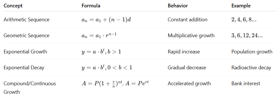
- Arithmetic sequence grows by constant addition, while a geometric sequence grows by constant multiplication. This distinction directly connects sequences to linear growth and exponential growth models, respectively.
- Arithmetic sequence example: 2,5,8,11…where d=3.
Formula: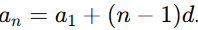
Source: Kapdec.com
- Geometric sequence example: 3,6,12,24… where r=2.
Formula: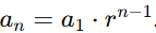
Source: Kapdec.com
Why important? Because exponential functions are essentially the continuous extension of geometric sequences, understanding sequences is the first step in analysing real-world growth and decay.
2. Explicit and Recursive Formulas
Sequences can be expressed in two ways:
- Explicit Formula gives a direct rule for finding any term in the sequence without knowing the previous terms.
Example: For geometric sequence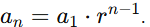
Source: Kapdec.com
- Recursive Formula defines each term based on its predecessor, requiring a starting value.
Example: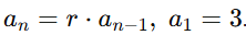
Source: Kapdec.com
Connection: Recursive formulas model processes that depend on the previous state (like population growth each year), while explicit formulas allow prediction without step-by-step calculation.
3. Geometric Sequences in Depth
Geometric sequences are central to growth modeling because they describe multiplicative change.
- General form:
Source: Kapdec.com
- Behavior depends on r:
- r>1: growth.
- 0<r<1: decay.
- r<0: alternating growth/decay (oscillation).
Example: A bacteria culture doubles every hour starting with 100.
Source: Kapdec.com
After 6 hours:
Source: Kapdec.com
This sequence acts as a discrete model for exponential growth.
4. Exponential Growth Models
Exponential functions represent continuous growth when the rate of change is proportional to the current value.
- Formula:
Source: Kapdec.com
- Distinguishing feature: growth accelerates over time instead of staying constant like linear functions.
Example: A city’s population of 500 grows at 8% yearly.
Source: Kapdec.com
Source: Kapdec.com
This example highlights how small percentages compound into large increases.
5. Exponential Decay Models
Exponential decay models situations where a quantity decreases at a rate proportional to its current amount.
- Formula:
Source: Kapdec.com
- Decay is never linear; instead, it slows over time but never fully reaches zero (asymptotic behavior).
Example: A radioactive substance loses 5% of its mass yearly, starting at 200 g.
Source: Kapdec.com
Source: Kapdec.com
This shows the gradual decline toward zero, illustrating natural decay processes.
Source: Kapdec.com
6. Compound Interest & Continuous Growth
Finance provides one of the clearest real-world uses of exponential growth.
- Compound Interest Formula:
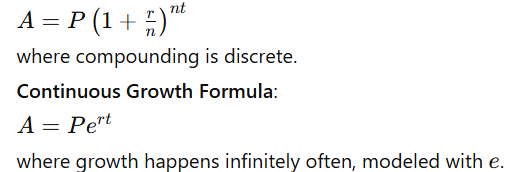
Source: Kapdec.com
Example: $1000 invested at 6% compounded monthly for 5 years:

Source: Kapdec.com
This highlights how frequency of compounding accelerates growth.
7. Connection Between Geometric Sequences & Exponential Functions
Geometric sequences can be seen as the discrete version of exponential functions.
- A geometric sequence like
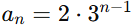
Source: Kapdec.com
that evaluates at natural numbers n.
- The corresponding exponential function
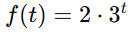
Source: Kapdec.com
is defined for all real t.
This relationship bridges the gap between step-by-step discrete growth and smooth continuous growth.
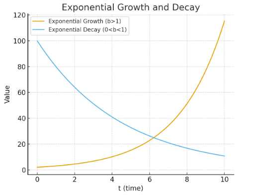
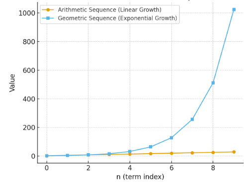
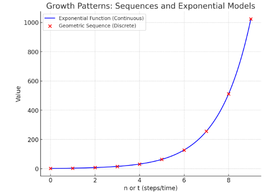
8. Graphical Representation of Exponential Functions
Graphs reveal behavior beyond formulas:
- Growth (b>1): curve rises steeply, has horizontal asymptote at y=0.
- Decay (0<b<1): curve declines but never reaches zero.
- Always positive if coefficient is positive.
Example:
- y=2x: passes (0,1), grows rapidly as x→∞.
- y= (1/2) x: passes (0,1), decays to 0 as x→∞.
Visualizing the graph helps understand long-term trends.
Source: Kapdec.com
9. Model Fitting with Data
Often, real-world data does not come as neat formulas, so exponential regression helps find the best-fit exponential model.
- Method: Use tools (calculator/software) to estimate parameters a and b for y=abx.
- Purpose: Predict unknown values, confirm if exponential is a good fit.
Example:
Bacteria counts:
Source: Kapdec.com
Source: Kapdec.com
The model captures multiplicative growth between each step.
10. Applications in Real-World Problems
Exponential models are universal:
- Finance: compound interest, inflation.
- Biology: population dynamics, disease spread.
- Physics: radioactive decay, half-life.
- Technology: Moore’s law (chip performance doubles periodically).
Example: Car depreciation: A $20,000 car loses 15% annually.
Source: Kapdec.com
Source: Kapdec.com
This demonstrates decay modeling in economics.
COMPARISON TABLE
Source: Kapdec.com
Source: Kapdec.com
Example: -Evaluate -12x3-1 dx
Source: Kapdec.com
Solution: x3 – 1 ≤ 0 on [–1, 0]
x3 – 1 ≤ 0 on [0, 1]
x3 – 1 ≥ 0 on [1, 2]
-12x3-1dx=-10–x3-1 dx+01–x3-1 dx+12x3-1 dx
Source: Kapdec.com
= –-10x3-1 dx-01x3-1 dx+12x3-1 dx
Source: Kapdec.com
= –x44-x-10–x44-x01+x44-x12
Source: Kapdec.com
= –0+54–-34-0+2--34
Source: Kapdec.com
= –54+34+114=94
Source: Kapdec.com
Five Conclusive Points
- Sequences lay the foundation – Arithmetic and geometric sequences help bridge discrete patterns with continuous functions.
- Exponential models capture real growth – They represent rapid change in population, finance, technology, and natural processes.
- Geometric sequences connect to exponentials – Discrete ratios extend naturally into continuous exponential functions.
- Graphical insights clarify behavior – Comparing sequences (dots) and exponentials (curves) highlights long-term trends and asymptotic limits.
- Applications validate the theory – From compound interest to radioactive decay, exponential models provide accurate, predictive power in real life.
Scan to visit this resource online
https://kapdec.com/resources/growth-patterns-sequences-and-exponential-models
