First & Second Order Test

Unit: Analytical Application of Differentiation

Chapter: First & Second Order Test

Reference: – Rolle’s Theorem, Intermediate value theorem, Extreme values, Critical points, Local extrema, Absolute extrema, closed intervals, First & Second derivative test, Concavity, Inflection points, Approximate values, Mean value theorem for integrals, Average value functions.

After studying this chapter, you should be able to:

Introduction to 1^st & 2^nd Order Derivatives.
Third & Higher Order Derivatives.
Notation & Representation of Functions.
Applications & Conclusion.

Introduction to 1^st & 2^nd Order Derivatives: –

First-order derivative:

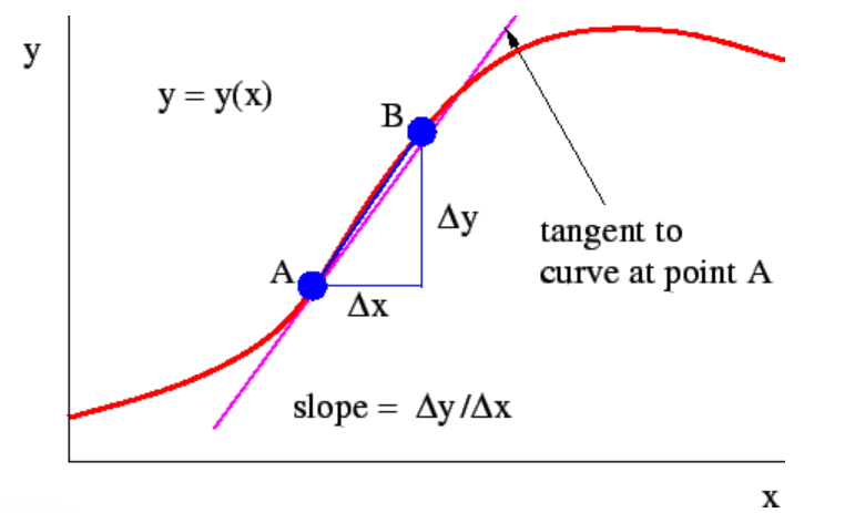
The first-order derivative of a function f(x), denoted as f'(x) or dy/dx, represents the rate of change of the function for the independent variable x at any given point.
Geometrically, the first derivative corresponds to the slope of the tangent line to the graph of the function at a particular point.
It provides information about the increasing or decreasing behavior of the function, as well as the critical points (where the derivative is zero or undefined) and the locations of relative extrema.
Calculating the first derivative involves applying various differentiation rules, such as the power rule, product rule, quotient rule, chain rule, and implicit differentiation.

Second-order derivative:

The second-order derivative of a function f(x), denoted as f''(x) or d²y/dx², is obtained by differentiating the first derivative of the function.
Geometrically, the second derivative indicates the concavity of the function's graph. It reveals whether the graph is concave up (opening upward) or concave down (opening downward) at a given point.
The second derivative can help identify points of inflection, which are points where the concavity of the function changes.
The sign of the second derivative (positive or negative) provides information about the increasing or decreasing behavior of the first derivative, and hence the original function.
Calculating the second derivative typically involves differentiating the first derivative using the differentiation rules.

(Representation of Derivatives)

3^rd & Higher Order Derivatives:

Third-order derivative:

The third-order derivative of a function f(x), denoted as f'''(x) or d³y/dx³, is obtained by differentiating the second-order derivative.
The third derivative provides additional information about the behavior of the function beyond what the first and second derivatives reveal.
Geometrically, the third derivative can help identify points of inflection where the concavity of the graph changes.
The sign of the third derivative can indicate the behavior of the second derivative, helping determine whether the concavity is increasing or decreasing.

Higher-order derivatives:

Higher-order derivatives can be obtained by differentiating the previous derivative multiple times. For example, the fourth derivative is obtained by differentiating the third derivative, and so on.
Higher-order derivatives provide increasingly detailed information about the function's behavior, including curvature, the rate of change of concavity, and higher-level trends.
These derivatives help in analyzing complex functions and understanding their intricate features, such as oscillations, turning points, and higher-order extrema.

Nested function & Multiple Variables: –

Nested Functions: Nested functions refer to functions that are composed together in a sequence, where the output of one function becomes the input of another.

Function Composition: When functions are nested, the output of the inner function serves as the input to the outer function. This composition allows for more complex transformations of variables.

Inner Function: The inner function refers to the function that is placed inside another function. It typically takes an independent variable as its input and produces an output.

Outer Function: The outer function refers to the function that contains the inner function. It takes the output of the inner function as its input and produces the final output of the nested function.

Variables in Nested Functions: When dealing with nested functions, it's important to consider the variables involved at different levels.

Independent Variable: The independent variable is typically associated with the innermost function. It represents the input to the nested function and is usually denoted as x.

Intermediate Variables: In a nested function, there can be intermediate variables between the inner and outer functions. These variables are generated during the evaluation of the inner function and serve as inputs to the outer function.

Dependent Variable: The dependent variable represents the final output of the nested function and is typically denoted as y.

Differentiation of Nested Functions: When differentiating a nested function, the chain rule is applied iteratively. The derivative of the outer function for its input is multiplied by the derivative of the inner function for its input, which can involve additional intermediate variables.

Order of Evaluation: When differentiating a nested function, it's important to evaluate the derivatives in the correct order, starting from the innermost function and moving outward.

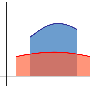
(Nested variable graph)

Notation & Representation of Inverse Functions: –

Implicit Functions: An implicit function is a function where the dependent and independent variables are not explicitly separated. In other words, the equation defining the function does not express y explicitly in terms of x.

Implicit Differentiation: Implicit differentiation is a technique used to find the derivatives of implicitly defined functions.

Procedure: To perform implicit differentiation, you treat the dependent variable y as a function of x and differentiate both sides of the equation for x. However, when differentiating y for x, you also need to consider the chain rule since y is not explicitly expressed in terms of x.

Chain Rule in Implicit Differentiation: When differentiating y for x, you apply the chain rule to the terms involving y. This involves multiplying the derivative of y for x (dy/dx) by the derivative of the term inside the brackets concerning y.

Simplification: After applying implicit differentiation, you can simplify the resulting equation to solve for dy/dx, which represents the derivative of the implicitly defined function.

Applications: Implicit differentiation is commonly used in various mathematical fields, such as physics and engineering, where relationships between variables are defined implicitly.

APPLICATIONS & CONCLUSIONS: –

Curve sketching: The first derivative helps identify critical points, relative extrema, and intervals of increasing or decreasing behavior. The second derivative assists in determining concavity and points of inflection. Collectively, these properties aid in drawing an accurate graph of the function.

Optimization problems: To find the maximum or minimum values of a function, critical points must be located. The first and second derivatives play a crucial role in solving optimization problems by providing information about the slope and concavity of the function.

Related rates: When two or more variables are related to each other, the derivatives help determine the rate at which one variable changes to another. The first derivative enables the calculation of rates of change, while the second derivative helps identify extreme rates or points of change in the rate of change.

Example: – Find the third-order derivative of the function f(x) = 2x³ – 3x² + 4x – 5.

Solution: – To find the third-order derivative, we will differentiate the function three times. Let's start with the first derivative:

Step 1: First-order derivative (f'(x)): f'(x) = d/dx (2x³ – 3x² + 4x – 5) = 6x² – 6x + 4

Now, let's move on to the second derivative:

Step 2: Second-order derivative (f''(x)): f''(x) = d/dx (6x² – 6x + 4) = 12x – 6

Finally, we'll differentiate the second derivative to find the third-order derivative:

Step 3: Third-order derivative (f'''(x)): f'''(x) = d/dx (12x – 6) = 12

So, the third-order derivative of f(x) = 2x³– 3x² + 4x – 5 is f'''(x) = 12.

Example:- Consider the function f(x) = x³ – 3x² – 9x + 5.

First-Order Test (First Derivative Test):

Find the critical points by setting the derivative equal to zero and solving for x: f'(x) = 3x² – 6x – 9 = 0. Factoring, we get: 3(x – 3)(x + 1) = 0. This gives us two critical points: x = 3 and x = -1.
Analyze the sign of the derivative around the critical points:
- For x < -1, choose x = -2 as a test point. Substitute it into f'(x): f'(-2) = 15 > 0.
- For -1 < x < 3, choose x = 0 as a test point. Substitute it into f'(x): f'(0) = -9 < 0.
- For x > 3, choose x = 4 as a test point. Substitute it into f'(x): f'(4) = 39 > 0.
Draw conclusions based on the significant changes of the derivative:
- At x = -1, the sign of the derivative changes from positive to negative. Therefore, there is a local maximum at x = -1.
- At x = 3, the sign of the derivative changes from negative to positive. Therefore, there is a local minimum at x = 3

Key Points

The first derivative measures the rate of change of a function at any given point.
It provides information about the slope and the increasing or decreasing behavior of a function.
The first derivative is used to find critical points, which are points where the derivative is zero or undefined.
Critical points can indicate potential local extrema or points of inflection in a function.
The first derivative is involved in the First Derivative Test, which helps determine the nature of critical points (maximum, minimum, or neither).
The sign of the first derivative (+, -, or zero) provides information about the intervals of increase and decrease of a function.
The first derivative can be used to identify relative extrema, where the function changes from increasing to decreasing or vice versa.
The first derivative can help analyze the behavior of a function near vertical asymptotes or vertical tangent lines.
The first derivative can be used to find the equations of tangent lines and to determine the direction of motion in applications such as velocity and rate of change problems.
The first derivative of a function f(x) is denoted as f'(x) or dy/dx.
The second derivative measures the rate of change of the first derivative, or the rate of change of the slope, at any given point.
It provides information about the concavity (upward or downward) of a function.
The second derivative is used to find points of inflection, which are points where the concavity of a function changes.
The second derivative is involved in the Second Derivative Test, which helps determine the nature of critical points (maximum, minimum, or neither) based on concavity.
The sign of the second derivative (+, -, or zero) provides information about the intervals of concave up and concave down of a function.
The second derivative can be used to find the equations of the normal lines to curves.
The second derivative can help identify possible points of inflection or changes in concavity.
The second derivative of a function f(x) is denoted as f''(x) or d^2y/dx^2.
The second derivative of a function can be obtained by differentiating the first derivative.
The second derivative can be used to analyze the behavior of a function near horizontal tangent lines or horizontal asymptotes.

Unit: Analytical Application of Differentiation

Chapter: First & Second Order Test

Most Read

Did you like this page?