Modeling Change With Parametric Functions

Unit: Functions involves Parameters, Vectors & Matrices

Chapter: Modeling Change with Parametric Functions

Reference: – Parametric equations, Parametric curves, Tangent lines, Normal lines, Arc length, Curvature, Acceleration, Tangent Vectors, Normal Vectors, Binormal vectors, Unit Tangent, Planar curves, Polar coordinates, Applications & Properties

After studying this chapter, you should be able to:

Introduction to Parametric & Vector-Valued Functions.
Tangent, Normal & Binormal Vectors.
Unit Tangent & Planar curves.
Polar coordinates, Applications & Properties.

Introduction to Parametric Functions

Parametric equations represent curves or objects in a plane by defining their coordinates as functions of an independent variable (usually denoted as t).
The independent variable t is often interpreted as time, representing how the curve or object changes over time.
Parametric equations typically consist of two or three equations that express the x, y (and sometimes z) coordinates of a point on the curve as functions of t.
Parametric equations allow for more flexibility in describing complex curves or motion compared to traditional Cartesian equations.
To graph a parametric curve, a table of values is often used to plot individual points by substituting different values of t into the equations.
The derivative of a parametric equation represents the rate of change of the x and y coordinates for t, often interpreted as the velocity vector.
The chain rule is used to find the derivatives of parametric equations by differentiating the x and y equations separately and then combining the results.
Tangent lines to a parametric curve can be found by evaluating the derivative at a specific value of t and determining the slope.
The slope of the tangent line at a given point on a parametric curve can be found using the derivative and represents the rate at which the curve is changing at that point.
The arc length of a parametric curve can be calculated using integrals and a specific formula that takes into account the derivative of the parametric equations.
Curvature is a measure of how sharply a curve is bending at a given point, and it can be determined using the derivatives of the parametric equations.
Parametric equations can be used to model various real-world scenarios, such as projectile motion, the motion of objects in space, or the path of a moving particle.

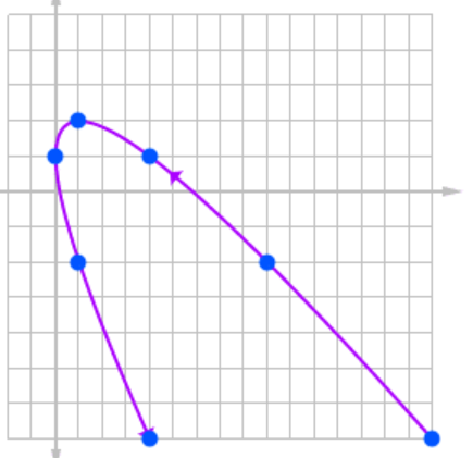
(Parametric Functions)

Introduction to Vector-Valued Functions: –

Vector-valued functions are functions that map a real number (usually denoted as t) to a vector in two or three-dimensional space.

Vector-valued functions are often used to describe the motion of objects in space or the path of a particle.

The components of a vector-valued function represent the coordinates of a point in space as functions of t.

The derivative of a vector-valued function represents the rate of change of the position vector for t, often interpreted as the velocity vector.

The derivative of a vector-valued function is found by differentiating each component of the function separately.

The chain rule is used to find the derivatives of vector-valued functions by applying the derivative to each component and combining the results.

The second derivative of a vector-valued function represents the rate of change of the velocity vector and is interpreted as the acceleration vector.

Tangent vectors to a vector-valued function can be found by evaluating the derivative at a specific value of t, representing the direction of motion at that point.

The magnitude of the derivative of a vector-valued function represents the speed or magnitude of the velocity vector.

The arc length of a vector-valued function can be calculated using integrals and a specific formula that takes into account the derivative of the vector-valued function.

Vector-valued functions can be used to model various real-world scenarios, such as the trajectory of a projectile, the motion of a particle, or the path of a moving object.

Vector-valued functions are also essential in studying topics such as curves in space, motion in three dimensions, and the fundamental principles of calculus in higher dimensions.

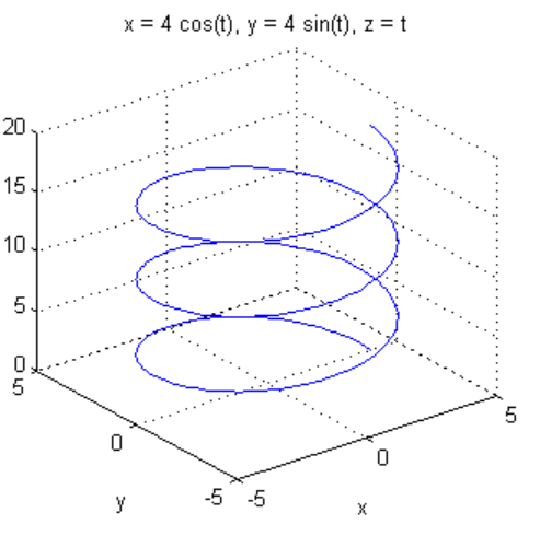
(Vector–Valued Function)

Tangent, Normal & Binormal Vectors

Tangent vectors represent the direction of motion or the instantaneous velocity of a curve or path at a specific point.

Tangent vectors are typically found by taking the derivative of a parametric or vector-valued function and evaluating it at a given point.

The tangent vector is parallel to the curve at the point of tangency and points in the direction of increasing t.

Normal vectors are perpendicular to the tangent vectors and represent the direction of the curve bending or the instantaneous curvature at a specific point.

Normal vectors can be obtained by taking the derivative of the tangent vector and normalizing it to have a magnitude of 1.

The normal vector is always orthogonal to the tangent vector and lies in the plane that the curve lies on.

The binormal vector is perpendicular to both the tangent vector and the normal vector and represents the "twisting" or "turning" of a curve in three-dimensional space.

The binormal vector can be obtained by taking the cross product of the tangent vector and the normal vector.

The binormal vector is always orthogonal to both the tangent vector and the normal vector, forming a three-dimensional orthogonal coordinate system known as the Frenet-Serret frame.

The Frenet-Serret formulas relate the derivatives of the tangent, normal, and binormal vectors to the curvature and torsion of a curve.

The curvature of a curve measures how sharply it bends at a given point and can be calculated using the derivatives of the tangent vector.

The torsion of a curve measures how much it twists in space and can be calculated using the derivatives of the tangent, normal, and binormal vectors.

Unit Tangent & Planar curves

The unit tangent vector is a vector of length 1 that represents the direction of motion or the direction of the curve at a specific point.

The unit tangent vector is obtained by normalizing the tangent vector and dividing it by its magnitude.

The unit tangent vector is always parallel to the tangent vector but has a magnitude of 1, providing only the direction information.

The unit tangent vector is useful in studying the behavior of curves without being influenced by the speed or magnitude of the motion.

Planar curves are curves that lie entirely in a single plane in three-dimensional space.

Planar curves can be described by parametric equations or vector-valued functions that have x and y coordinates but no z coordinate.

The unit tangent vector is also useful in analyzing planar curves as it represents the direction of motion on the plane.

The curvature of a planar curve measures how sharply it bends at a given point and can be calculated using the derivatives of the unit tangent vector.

The curvature of a planar curve is related to the rate of change of the unit tangent vector for arc length.

The unit normal vector is a vector that is orthogonal to the tangent vector and lies in the plane of the curve.

The unit normal vector can be obtained by normalizing the derivative of the unit tangent vector or by taking the derivative of the tangent vector and normalizing it.

The unit normal vector provides information about the direction of the curve's curvature or the direction the curve is turning in the plane.

Polar Co-ordinates & Applicative Properties

Polar coordinates are an alternative coordinate system to Cartesian coordinates, representing points in a plane using a distance from the origin (r) and an angle from the positive x-axis (θ).

The radial distance (r) in polar coordinates represents the length from the origin to a point, and it can be either positive or negative.

The angle (θ) in polar coordinates represents the counterclockwise rotation from the positive x-axis to the line connecting the origin and the point.

Converting between Cartesian coordinates (x, y) and polar coordinates (r, θ) involves using trigonometric functions such as sine and cosine.

Polar equations are equations that relate the distance (r) and angle (θ) in polar coordinates. They can describe curves, shapes, or regions in a plane.

Polar curves can have different symmetries and can take the form of lines, circles, spirals, or more complex shapes.

Derivatives of polar equations can be found by using the chain rule and trigonometric identities.

The area of a region bounded by a polar curve can be determined using integration and a specific formula that takes into account the angle and radius.

Polar coordinates are particularly useful in analyzing and describing curves with rotational symmetry or radial growth patterns.

Applications of polar coordinates in calculus include studying the motion of objects following circular paths, analyzing periodic phenomena, and solving problems involving polar symmetry.

Polar coordinates can be used to model and analyze phenomena such as planetary orbits, pendulum motion, or the behavior of waves.

Understanding polar coordinates and their applications is important in various branches of science and engineering, such as physics, astronomy, and engineering design.

Example: – Find the derivative of the parametric equations x = 2t² and y = t – 1.

Solution:

To find the derivative, we differentiate each equation for t:

dx/dt = d(2t²)/dt = 4t,

dy/dt = d(t – 1)/dt = 1.

Therefore, the derivative of the parametric equations is given by the vector-valued function:

r'(t) = 4t i + j.

Example: – Consider the vector-valued function r(t) = (2t, t², 3t – 1). Find the derivative of r(t).

Solution:

To find the derivative, we differentiate each component of the vector-valued function for t:

dr/dt = (d(2t)/dt, d(t²)/dt, d(3t – 1)/dt)

= (2, 2t, 3).

Therefore, the derivative of the vector-valued function is given by the vector-valued function:

r'(t) = (2, 2t, 3).

Key Points

Parametric functions represent curves or objects in a plane by defining their coordinates as functions of an independent variable (usually denoted as t).

Vector-valued functions are functions that map a real number (usually denoted as t) to a vector in two or three-dimensional space.

The derivative of a parametric or vector-valued function represents the rate of change of the position vector for the independent variable (t).

To find the derivative of a parametric function, you differentiate each component of the function for t.

The chain rule is used when differentiating parametric or vector-valued functions. It involves differentiating each component and then combining the results.

The derivative of a parametric or vector-valued function is itself a vector-valued function.

The derivative of a parametric or vector-valued function gives the velocity vector, which represents the instantaneous rate of change and the direction of motion.

The second derivative of a parametric or vector-valued function represents the rate of change of the velocity vector and is interpreted as the acceleration vector.

Tangent vectors to a parametric or vector-valued function can be found by evaluating the derivative at a specific value of t, representing the direction of motion at that point.

The magnitude of the derivative of a parametric or vector-valued function represents the speed or magnitude of the velocity vector.

The derivative of a vector-valued function can be interpreted as the velocity vector, which provides information about the rate and direction of motion.

The derivative of a vector-valued function can be used to find tangent lines, tangent planes, or instantaneous rates of change in applications.

The derivative of a parametric or vector-valued function can be used to determine the curvature of a curve at a given point.

The derivative of a parametric or vector-valued function can be used to find the arc length of a curve or the length of a displacement vector.

Understanding the derivatives of parametric and vector-valued functions is crucial for studying motion, curve analysis, and solving real-world problems involving time-varying quantities.

Unit: Functions involves Parameters, Vectors & Matrices

Chapter: Modeling Change with Parametric Functions

Most Read

Did you like this page?