KAPDEC® | Elite STEM Learning Platform | https://kapdec.com
Unit: Exploring Two – Variable Data
Chapter: Linear Regression Models & Residual plots
Reference: – Simple Linear Regression, Slope & Intercept, Residual & Residual Plots, Positive & Negative Residuals, Assumptions of Linear Regressions, Linearity & Normality, Influential points & Outliers, Transformations & Non-linear relationships, Coefficient of Determination, Model Assessment & Inference, Applications.
After studying this chapter, you should be able to understand:
- Simple Linear Regression & Residual Plots.
- Assumptions of Linear Regressions, Positive-Negative residuals.
- Influential points & Outliers, Slope & Intercept.
- Coefficient of determination, Model Assessment & Inference
Simple Linear Regression & Residual Plots
Simple Linear Regression:
- Definition: Simple Linear Regression is a statistical method used to model the relationship between a dependent variable (response) and a single independent variable (predictor) using a linear equation.
- Equation: The linear regression equation is represented as: y = b₀ + b₁x + ε, where y is the dependent variable, x is the independent variable, b₀ is the y-intercept, b₁ is the slope, and ε represents the error term.
- Objective: The goal of simple linear regression is to find the best-fitting line (regression line) that minimizes the sum of squared residuals, which are the vertical differences between observed and predicted values.
- Least Squares Criterion: The method used to find the best-fitting line by minimizing the sum of squared residuals is known as the Least Squares Criterion.
- Assumptions: Linear regression assumes that the relationship between the variables is linear, the errors are normally distributed, the errors have constant variance (homoscedasticity), and the errors are independent.
- Coefficient Interpretation: The slope coefficient (b₁) indicates the change in the dependent variable for a one-unit change in the independent variable, assuming all other variables are held constant.
- Coefficient of Determination (R²): R² measures the proportion of the total variability in the dependent variable that is explained by the regression model. It ranges from 0 to 1, where higher values indicate a better fit.
- Hypothesis Testing: Hypothesis tests can be performed to determine if the slope coefficient is significantly different from zero. This involves testing whether the predictor has a significant effect on the response.
Residual Plots:
- Definition: Residual plots are graphical representations of the differences between observed and predicted values (residuals) in a regression analysis.
- Purpose: Residual plots help to assess the appropriateness of a linear regression model by identifying patterns or deviations in the residuals that could indicate violations of assumptions or non-linearity.
- Homoscedasticity: A scatter plot of residuals against the predicted values can help assess homoscedasticity. A consistent spread of residuals around zero indicates constant variance, while a funnel shape suggests heteroscedasticity.
- Linearity: A residual plot of residuals against the predictor variable can help check for linearity. A random distribution of points around zero suggests linearity, while patterns suggest non-linearity.
- Normality: A histogram or a Q-Q plot of residuals can help assess the normality assumption. A bell-shaped histogram and points along the diagonal line in a Q-Q plot indicate normality.
- Outliers and Influential Points: Residual plots can reveal outliers (residuals far from zero) and influential points (residuals that significantly affect the regression line when removed).
- Residual Patterns: Patterns in residual plots, such as curves, clusters, or changing spreads, may indicate issues with the model, such as omitted variables or heteroscedasticity.
- Ideal Residual Plot: In an ideal case, a residual plot should show random scatter of points around zero, indicating that the linear regression assumptions are met and the model is appropriate.
Assumptions of Linear Regressions, Positive-Negative residuals
Assumptions of Linear Regression:
- Linearity: The relationship between the dependent variable and the predictor(s) is assumed to be linear. This means that the change in the response variable is constant for each unit change in the predictor variable.
- Independence: The residuals (errors) should be independent of each other. In other words, the value of one residual should not provide information about the value of another residual.
- Normality: The residuals should be normally distributed. This assumption is important for hypothesis testing and constructing confidence intervals.
- Equal Variance (Homoscedasticity): The variability of the residuals should be roughly constant across all levels of the predictor variable. This ensures that the spread of residuals is consistent, indicating that the model is suitable for the entire range of data.
- No Multicollinearity: In multiple regression, predictor variables should not be highly correlated with each other. Multicollinearity can lead to unstable and unreliable coefficient estimates.
- No Autocorrelation: The residuals should not exhibit any patterns or correlation over time or space. Autocorrelation can occur in time series or spatial data and indicates that the model is not capturing all relevant information.
- Zero Mean Residuals: The sum of the residuals should be approximately zero, indicating that the model’s predictions are, on average, accurate.
Positive-Negative Residuals:
- Definition: Residuals are the differences between observed and predicted values. Positive residuals occur when observed values are higher than predicted values, while negative residuals occur when observed values are lower than predicted values.
- Interpretation of Positive Residuals: Positive residuals suggest that the model tends to underestimate the actual values. This could be due to an omitted predictor variable or a non-linear relationship.
- Interpretation of Negative Residuals: Negative residuals indicate that the model tends to overestimate the actual values. Similar to positive residuals, this could be due to model deficiencies.
- Ideal Scenario: In a well-fitting linear regression model, positive and negative residuals should be randomly distributed around zero with no discernible pattern.
- Residual Plots: Positive and negative residuals can be visualized using residual plots. These plots help identify patterns or trends in the residuals that might indicate problems with the model.
- Impact on Coefficient Estimates: Positive and negative residuals can affect the estimates of the regression coefficients, potentially leading to biased results.
- Outliers and Influential Points: Both positive and negative residuals can be indicators of outliers or influential points in the data. These points may disproportionately affect the model’s fit and assumptions.
- Model Improvement: If a linear regression model consistently exhibits either positive or negative residuals, it may be necessary to revisit the model’s assumptions, check for omitted variables, or consider more complex modeling techniques.
Influential points & Outliers, Slope & Intercept
Influential Points & Outliers:
- Influential Points: Influential points are individual data points that have a significant impact on the results of a statistical analysis, such as regression models. These points can strongly affect the slope, intercept, and overall fit of the model.
- Outliers: Outliers are data points that deviate significantly from the overall pattern of the data. They can be influential if they have a disproportionate impact on the model’s parameters.
- Impact on Slope and Intercept: Outliers and influential points can greatly affect the estimated slope and intercept of a regression line. In particular, outliers can pull the line towards them, altering the overall trend.
- Leverage: Leverage measures how far a data point’s predictor value is from the mean predictor value. Points with high leverage can have a large influence on the slope of the regression line.
- Cook’s Distance: Cook’s Distance is a statistical measure used to identify influential points. Large Cook’s Distance values indicate points that significantly affect the regression parameters.
- Residuals and Outliers: Outliers often result in large residuals, as they don’t fit the model well. However, not all large residuals are influential, and not all outliers are influential either.
- Influential Points in Context: It’s important to consider the context of the data and the study when identifying influential points. Some outliers might be valid data points, while others could be errors.
- Handling Influential Points: Depending on the circumstances, influential points can be removed, transformed, or analyzed separately to assess their impact on the model.
Slope & Intercept:
- Slope (Coefficient): In a linear regression equation (y = b₀ + b₁x), the slope (b₁) represents the change in the dependent variable (y) for a one-unit change in the independent variable (x).
- Interpretation of Slope: The slope indicates the rate of change in the dependent variable per unit change in the independent variable. A positive slope suggests a positive correlation, while a negative slope suggests a negative correlation.
- Intercept (Constant Term): In the linear regression equation, the intercept (b₀) is the value of the dependent variable when the independent variable is zero.
- Interpretation of Intercept: The intercept provides the starting point of the regression line on the y-axis. It may or may not have a meaningful interpretation depending on the context.
- Effect of Slope and Intercept on Regression Line: The slope determines the steepness of the regression line, while the intercept determines where the line crosses the y-axis.
- Changing Slope and Intercept: Altering the slope and intercept can change the position and angle of the regression line, affecting its fit to the data.
- Regression Equation: The complete regression equation specifies how changes in the independent variable(s) lead to changes in the dependent variable. It includes both the intercept and the slope.
- Assumptions and Interpretation: When interpreting the slope and intercept, it’s important to consider the assumptions of linear regression, such as linearity, independence, and homoscedasticity.
Coefficient of determination, Model Assessment & Inference
Coefficient of Determination:
- Definition: The Coefficient of Determination (R²) is a statistical measure that indicates the proportion of the variability in the dependent variable (response) that is explained by the independent variable(s) (predictor(s)) in a regression model.
- Interpretation: R² ranges from 0 to 1. A higher R² indicates that a larger proportion of the variability in the response is accounted for by the model’s predictors.
- Calculation: R² is calculated as the ratio of the explained sum of squares (SSR) to the total sum of squares (SST), often expressed as a percentage.
- Meaning of R² Values: An R² close to 1 suggests a strong relationship between the variables, while an R² close to 0 suggests a weak relationship. However, a high R² doesn’t necessarily imply causation.
- Limitations: R² does not provide information about the quality of the model’s predictions outside the observed data range, and it doesn’t indicate the direction or shape of the relationship.
- Goodness of Fit Tests: Goodness of fit tests help assess how well the model fits the data. Common tests include the F-test for overall model fit and individual t-tests for the significance of coefficients.
- Residual Analysis: Residual plots are used to evaluate the assumptions of the model, such as linearity, independence, and homoscedasticity. Patterns in the residuals may suggest problems with the model.
- Cross-Validation: Cross-validation techniques, such as k-fold cross-validation, assess the model’s performance by partitioning the data into training and testing sets, helping to gauge its predictive accuracy.
- Overfitting and Underfitting: Overfitting occurs when the model fits the training data too closely, leading to poor generalization to new data. Underfitting results in a model that is too simplistic to capture the underlying patterns.
- Bias-Variance Trade-off: Model assessment involves managing the trade-off between bias (error due to overly simplistic models) and variance (error due to overcomplicated models).
Inference in AP Statistics:
- Hypothesis Testing: Hypothesis tests assess the significance of regression coefficients. The t-test is commonly used to determine if a coefficient is significantly different from zero.
- Confidence Intervals: Confidence intervals provide a range of plausible values for a population parameter (e.g., slope or intercept) based on sample data. A wider interval indicates more uncertainty.
- Degrees of Freedom: Degrees of freedom reflect the number of independent pieces of information available for estimating a parameter. In a regression, they affect the t-distribution used in hypothesis testing.
- p-value: The p-value indicates the strength of evidence against the null hypothesis. A small p-value (typically ≤ 0.05) suggests that the null hypothesis should be rejected.
- Type I and Type II Errors: In hypothesis testing, a Type I error occurs when a true null hypothesis is incorrectly rejected, and a Type II error occurs when a false null hypothesis is not rejected.
- ANOVA: Analysis of Variance (ANOVA) tests assess the significance of differences between group means. In regression, ANOVA is used to compare the full model to a reduced model without predictors.
- Multiple Comparisons: When conducting multiple hypothesis tests simultaneously, adjustments (e.g., Bonferroni correction) are made to control the familywise error rate.
- Assumptions: Inference relies on the assumptions of normality, independence, and constant variance. Violations of these assumptions may affect the validity of the results.
Example: Simple Linear Regression and Residual Plots
Suppose a researcher is interested in studying the relationship between the number of hours students spend studying (independent variable, x) and their scores on a math test (dependent variable, y). The researcher collects data from a sample of 10 students and wants to perform a simple linear regression analysis.
Here are the data points (hours studied, test score):
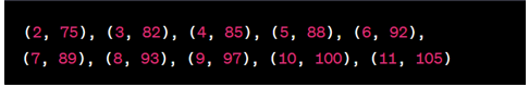
Source: Kapdec.com
Solution: – Step 1: Calculate the Regression Line
- Calculate the means:
- Mean of x (hours studied) = (2 + 3 + 4 + 5 + 6 + 7 + 8 + 9 + 10 + 11) / 10 = 6.5
- Mean of y (test score) = (75 + 82 + 85 + 88 + 92 + 89 + 93 + 97 + 100 + 105) / 10 = 91.6
- Calculate the slope (b₁):
- Using the formula: b₁ = Σ((xi – x̄)(yi – ȳ)) / Σ((xi – x̄)²)
- where xi is each value of x, x̄ is the mean of x, yi is each value of y, and ȳ is the mean of y.
Create a scatter plot of x (hours studied) against the residuals.
Interpretation: Follow
In the residual plot, if the points are randomly scattered around the horizontal line at y = 0, it indicates that the assumptions of the linear regression are satisfied. Deviations from randomness, such as patterns or trends in the residuals, may suggest violations of assumptions like linearity, homoscedasticity, or normality.
Scan to visit this resource online
https://kapdec.com/resources/linear-regression-models-residual-plot
