Unit: Systems of Two Linear Equations with Two Variables
Solution Techniques: Substitution, Elimination And Standard Rules
Overview
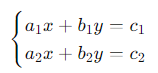
A system of two linear equations with two variables is a set of equations where each equation is linear and involves two variables, typically x and y. The general form of such a system is:
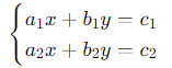
where a1, b1, c1, a2, b2, and c2 are constants.
Solutions to the System
The solution to a system of two linear equations can be:
- One unique solution: The lines intersect at a single point.
- No solution: The lines are parallel and do not intersect.
- Infinitely many solutions: The lines coincide (are the same line).
Methods of Solving
- Graphical Method:
- Plot both equations on the same set of axes.
- The point of intersection, if any, is the solution.
- If the lines are parallel, there is no solution.
- If the lines coincide, there are infinitely many solutions.
- Substitution Method:
- Solve one of the equations for one variable in terms of the other.
- Substitute this expression into the other equation.
- Solve the resulting single-variable equation.
- Substitute back to find the other variable.
- Elimination (Addition) Method:
- Multiply one or both equations by suitable constants to align coefficients.
- Add or subtract the equations to eliminate one variable.
- Solve the resulting single-variable equation.
- Substitute back to find the other variable.
- Matrix Method (using Determinants):
- Represent the system as a matrix equation AX=B.
- Use the inverse of the coefficient matrix A to solve for X, if A is invertible.
- X=A−1B.
Example Problem
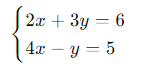
Consider the system:
Graphical Method:
- Convert to slope-intercept form (if necessary) and plot the lines.
- Determine the intersection point.
Substitution Method:
- Solve the second equation for y:
- y=4x−5
- Substitute into the first equation:
- 2x+3(4x−5)=6
- 2x+12x−15=6
- 14x=21
- x=
 =1.5
=1.5
- Substitute x=1.5 back into y=4x−5:
- 𝑦=4(1.5)−5=6−5=1
- Solution: (1.5,1)
Elimination Method:
- Align coefficients for elimination:
- Multiply the first equation by 1 and the second by 3:
- 2x+3y=6
- 12x−3y=15
- Add the equations:
- 14x=21
- x=1.5
- Substitute x=1.5 into the first equation to find 𝑦y:
- 2(1.5)+3y=6
- 3+3y=6
- 3y=3
- y=1
- Solution: (1.5,1)
Special Cases
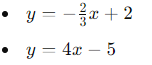
- Parallel Lines:
- The system
has no solution since the lines have the same slope but different y-intercepts.
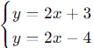
- Coincident Lines:
- The system
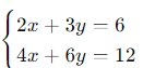
has infinitely many solutions since the second equation is a multiple of the first.
Determinant Method (Cramer's Rule)
Cramer's Rule is a mathematical theorem used to solve systems of linear equations with as many equations as unknowns, provided the system's determinant is non-zero. Here, we'll focus on using Cramer's Rule for systems of two linear equations with two variables.
System of Equations
Consider the system:
Determinants
To use Cramer's Rule, we need to calculate three determinants:
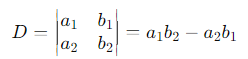
- Determinant D: This is the determinant of the coefficient matrix.
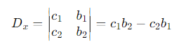
- Determinant Dx: This is the determinant of the matrix obtained by replacing the x-coefficients with the constants from the right-hand side of the equations.
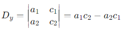
- Determinant Dy: This is the determinant of the matrix obtained by replacing the y-coefficients with the constants from the right-hand side of the equations.
Steps to Apply Cramer's Rule
- Determinant D:
- Determinant Dx:
- Determinant Dy:
- Solve for 𝑥x and 𝑦y:
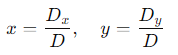
Provided 𝐷≠0, the system has a unique solution.
Summary
One unique solution: Lines intersect at one point.
No solution: Lines are parallel.
Infinitely many solutions: Lines coincide.
Methods include graphical, substitution, elimination, and matrix methods.
Special cases highlight the nature of solutions based on the relationship between the lines.
Understanding these fundamentals enables solving and analyzing systems of linear equations in various contexts.
Cramer's Rule provides a straightforward method to solve a system of linear equations using determinants, provided the determinant of the coefficient matrix is non-zero. The steps involve calculating the determinant of the coefficient matrix and two modified matrices, then using these determinants to find the values of the variables.