Represent & Statistics For 2 Categorical Variables

Unit: Exploring Two – Variable Data

Chapter: Represent & Statistics for 2 Categorical Variables

Reference: – Two-way Tables, Constructing & Interpreting, Marginal & Conditional frequencies, Joint, Marginal & Conditional distribution, Segmented Bar chart & Stacked Bar chart, Relative Risk & Odds Ratio, Independence & Association of Data, Conditional Probability & Independence, Simpson’s Paradox, Categorical Data Analysis, Applications.

After studying this chapter, you should be able to:

• Contingency Tables, Marginal & Conditional frequencies.
• Segmented & Stacked Bar chart, Relative & Odds Ratio.
• Conditional Probability & Simpson’s Paradox.
• Categorical data Analysis & Applications

Contingency Table & Marginal Frequencies

1. Two-Way Tables (Contingency Tables):

• • Two-way tables are used to organize categorical data for two variables.
  • They help identify patterns and relationships between variables.
  • Totals in the table provide information about the overall distribution.
  • Cells represent counts, frequencies, or percentages of observations.
  • The row and column totals provide marginal distributions.
  • Joint frequencies in specific cells show how the two variables relate.
  • Two-way tables can be used to calculate conditional probabilities.
  • Chi-squared tests can determine if variables are independent or associated.
  • Two-way tables are a foundation for more advanced analyses like logistic regression.
  • They are useful for exploring interactions in experimental designs.

1. Joint, Marginal, and Conditional Distributions:
   • Joint distribution shows the combined probabilities of two events.
   • Marginal distributions display probabilities for individual variables.
   • Summing across rows or columns provides marginal probabilities.
   • Conditional distributions focus on probabilities within specific conditions.
   • Conditional probabilities are calculated using joint and marginal probabilities.
   • Conditional distributions reveal how variables interact under certain conditions.
   • Marginal and joint probabilities can be used to calculate expected values.
   • Understanding these distributions is essential for Bayesian probability.
   • They play a role in constructing probability trees and decision analysis.
   • Conditional distributions are foundational in Bayesian statistics.

1. Segmented Bar Charts and Stacked Bar Charts:
   • Segmented bar charts visually compare frequencies or percentages.
   • They allow for easy comparison of subcategories within each variable.
   • Stacked bar charts display the composition of a whole across variables.
   • Each segment's height represents the proportion within a category.
   • Stacked bar charts reveal how parts contribute to the whole.
   • They help visualize both the total and relative distributions.
   • These charts can aid in detecting patterns and trends.
   • They are particularly useful for comparing distributions across groups.
   • Stacked bar charts can also represent cumulative percentages.
   • Both chart types are valuable tools for data communication.

1. Relative Risk and Odds Ratio:
   • Relative risk assesses the likelihood of an event occurring in one group versus another.
   • It measures the strength of association between categorical variables.
   • A relative risk of 1 indicates no association, less than 1 suggests lower risk, and greater than 1 suggests higher risk.
   • Relative risk is widely used in epidemiology and medical research.
   • Odds ratio compares the odds of an event happening in one group to another.
   • It's particularly useful in case-control studies and logistic regression.
   • An odds ratio of 1 implies no association, less than 1 implies lower odds, and greater than 1 implies higher odds.
   • Both measures are crucial for understanding risk factors and treatment effects.
   • Interpretation varies based on context and field of study.
   • Both measures aid in decision-making and policy formulation.

1. Independence and Association:
   • Independence means that the occurrence of one event does not affect the occurrence of the other.
   • An association suggests a relationship or connection between variables.
   • Chi-squared tests assess whether an association is statistically significant.
   • A low p-value indicates evidence against independence.
   • Cramer's V statistic quantifies the strength of association.
   • Association does not imply causation; confounding factors must be considered.
   • Understanding independence helps prevent drawing incorrect conclusions.
   • Associations can be positive, negative, or null.
   • Visualizing associations helps in communicating findings effectively.
   • Recognizing associations aids in making informed decisions.

1. Conditional Probability and Independence:
   • Conditional probability accounts for information about another event.
   • It's calculated as the probability of one event given the occurrence of another.
   • Independence of two events means that the occurrence of one does not affect the other's probability.
   • Conditional independence indicates that knowing one event occurred does not change the probability of the other event.
   • Conditional probability is foundational in Bayesian statistics.
   • Conditional independence assumptions are crucial in many statistical models.
   • Bayes' theorem is a key concept involving conditional probability.
   • Understanding conditional probability is essential for risk assessment.
   • Conditional distributions allow for more nuanced analysis.
   • Conditional probability is widely applied in fields like finance, biology, and social sciences.

1. Simpson's Paradox:
   • Simpson's Paradox occurs when a trend appears in different groups but disappears or reverses when the groups are combined.
   • It highlights the importance of considering lurking variables.
   • Simpson's Paradox emphasizes the dangers of drawing conclusions from aggregated data alone.
   • It challenges intuition and underscores the need for careful analysis.
   • Real-world examples include educational outcomes, medical studies, and voting patterns.
   • Analyzing subgroups separately is essential to avoid misleading interpretations.
   • Simpson's Paradox demonstrates the complexity of relationships between variables.
   • It underscores the importance of transparency in data reporting.
   • Identifying and understanding the paradox leads to more accurate conclusions.
   • Addressing Simpson's Paradox can inform better decision-making.

1. Categorical Data Analysis:
   • Categorical data analysis involves summarizing and interpreting data with categorical variables.
   • Techniques include frequency tables, bar charts, and contingency tables.
   • It helps uncover patterns, trends, and relationships in the data.
   • Categorical data analysis is fundamental in exploratory data analysis (EDA).
   • It's used in hypothesis testing, model building, and prediction.
   • Chi-squared tests are a cornerstone of categorical data analysis.
   • It's applicable in various fields, such as marketing, social sciences, and public health.
   • Proper analysis requires consideration of data quality and context.
   • Interpretation skills are crucial for drawing meaningful insights.
   • Categorical data analysis informs decision-making and policy recommendations.

1. Case Studies and Practical Applications:
   • Case studies provide real-world context for applying statistical concepts.
   • They bridge theory with practical problem-solving.
   • Analyzing actual data builds analytical skills and critical thinking.
   • Case studies showcase the relevance of statistics in various domains.
   • They demonstrate the importance of data-driven decision-making.
   • Practical applications include marketing analysis, medical research, and quality control.
   • Case studies encourage students to formulate hypotheses and draw conclusions.
   • They promote effective communication of findings and results.
   • Case studies highlight ethical considerations in data analysis.
   • Practical applications prepare students for data-related careers and research.

Example:

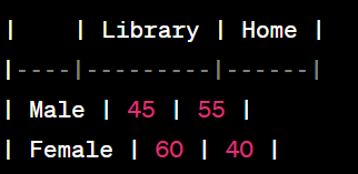
Suppose you are conducting a survey at a high school to understand the preferences of students regarding their study locations. You ask each student whether they prefer to study in the library or at home, and you also collect information about their gender. You want to determine if there is an association between the students' preferred study location and their gender.

Here's a sample of the collected data:

Solution:

1. Two-Way Table:

1. Marginal Distributions:
   • Marginal distribution of study location: Library (105), Home (95)
   • Marginal distribution of gender: Male (100), Female (100)
2. Segmented Bar Chart: (Visualization showing the preferences of male and female students for study locations)
3. Relative Risk and Odds Ratio:
   • Relative Risk = (Probability of Library Preference for Males) / (Probability of Library Preference for Females)
   • Odds Ratio = (Odds of Library Preference for Males) / (Odds of Library Preference for Females)
4. Independence and Association:
   • Perform a chi-squared test to assess whether study location preference and gender are independent.
5. Conditional Probability and Independence:
   • Calculate conditional probabilities, e.g., P(Home | Male) and P(Library | Female).
6. Simpson's Paradox:
   • Examine whether the relationship between study location and gender changes when considering subgroups (e.g., within male and female groups).
7. Categorical Data Analysis:
   • Summarize findings, discuss trends, and draw conclusions about the association between study location preference and gender.
8. Case Study and Practical Application:
   • Use the analysis to provide recommendations for creating conducive study environments based on gender preferences.

Key Points

• Two-Way Tables: Two-way tables organize categorical data for two variables, displaying counts or frequencies in cells.
• Joint, Marginal, and Conditional Distributions: Joint distribution combines two variables, while marginal and conditional distributions focus on one variable.
• Segmented Bar Charts: Segmented bar charts visually compare distributions of subcategories within each variable.
• Stacked Bar Charts: Stacked bar charts show composition of a whole by stacking segments representing categories.
• Relative Risk and Odds Ratio: These measures assess the strength of association between two categorical variables.
• Independence and Association: Independence means no relationship, while association indicates a relationship between variables.
• Chi-Squared Test: Determines if two categorical variables are independent or associated.
• Conditional Probability: Calculates probability of an event given another has occurred, key in Bayesian analysis.
• Simpson's Paradox: A trend in subgroups can reverse or disappear when groups are combined, highlighting lurking variables.
• Contingency Table Analysis: Involves calculating expected counts, chi-squared statistics, and degrees of freedom.
• Interpreting P-Values: A low p-value suggests evidence against independence, supporting an association.
• Contingency Coefficient and Cramer's V: Measures strength of association in contingency tables.
• Cross-Tabulation: Arranging data in a table to explore relationships between categorical variables.
• Conditional Independence: Knowing the value of one variable doesn't affect the probability of another, vital in modeling.
• Practical Applications: Analyzing real-world data helps understand relationships and informs decision-making.