Unit: Inference for Categorical Data: Chi – Square
Chapter: Chi- square Test for Homogeneity
Reference: – Categorical Data, Contingency tables, Expected & Observed frequencies, Hypothesis testing, Degree of freedom, Chi- square Statistics, Critical value, P value, Assumptions & Interpretations, Applications.
After studying this chapter, you should be able to:
- Categorical Data & Contingency Tables.
- Hypothesis Testing & Degree of Freedom.
- Chi – square test statistics & Critical Value.
- P Value & Interpretations.
Categorical Data & Contingency Tables
Categorical Data:
- Categorical data, also known as qualitative or nominal data, consists of observations that can be sorted into distinct categories or groups.
- Categorical variables have values that are labels or names, and they cannot be ordered or measured on a numerical scale.
- Examples of categorical data include gender (male/female), eye color (blue/brown/green), and type of car (sedan/SUV/truck).
- Categorical data is often presented in frequency tables or bar charts to show the distribution of observations among different categories.
- Definition: A contingency table is a way to organize categorical data from two or more groups or populations to analyze the association between two categorical variables.
- Rows and Columns: Contingency tables have rows representing different groups or populations, and columns representing categories or levels of another variable.
- Cell Entries: Each cell in the contingency table contains the frequency or count of observations falling into a specific combination of categories.
- Expected Frequencies: In the context of the Chi-Square Test for Homogeneity, expected frequencies are calculated assuming that the distribution of the categorical variable is the same across all groups.
- Null Hypothesis: The null hypothesis for the Chi-Square Test for Homogeneity states that there is no significant difference in the distribution of the categorical variable across the groups.
- Alternative Hypothesis: The alternative hypothesis suggests that there is a significant difference in the distribution of the categorical variable among the groups.
- Degrees of Freedom: The degrees of freedom for the Chi-Square Test for Homogeneity depend on the number of groups and categories and are used to determine the critical value or p-value.
- Test Statistic: The Chi-Square test statistic is calculated by comparing the observed frequencies in the contingency table to the expected frequencies under the null hypothesis.
- Calculation: The formula for the Chi-Square test statistic involves summing the squared differences between observed and expected frequencies, divided by the expected frequencies.
- Critical Value: The critical value is determined based on the chosen significance level and the degrees of freedom. It helps decide whether to reject the null hypothesis.
- P-Value: The p-value associated with the Chi-Square test statistic is used to assess the strength of evidence against the null hypothesis. A lower p-value suggests stronger evidence against the null hypothesis.
- Interpretation: The Chi-Square Test for Homogeneity results are interpreted by comparing the p-value to the significance level. If the p-value is below the significance level, you may reject the null hypothesis and conclude that there is a significant difference in the distribution of the categorical variable across groups.
Hypothesis Testing & Degree of Freedom
Hypothesis Testing:
- Purpose: Hypothesis testing is a fundamental concept in statistics used to make inferences about population parameters based on sample data.
- Null Hypothesis (H0): The null hypothesis is a statement of no effect or no difference. It serves as the default assumption to be tested against an alternative hypothesis.
- Alternative Hypothesis (Ha): The alternative hypothesis states the specific effect or difference you are trying to find evidence for. It contrasts with the null hypothesis.
- Significance Level (α): The significance level is the threshold below which you consider the evidence strong enough to reject the null hypothesis. Common levels include 0.05 and 0.01.
- P-Value: The p-value is a measure of the strength of evidence against the null hypothesis. A smaller p-value suggests stronger evidence against the null.
- Test Statistic: A test statistic is a calculated value that measures how far the sample data deviates from what is expected under the null hypothesis.
- Critical Value: The critical value(s) define the boundary beyond which you would reject the null hypothesis based on the chosen significance level. It is often used in comparison with the test statistic.
- Type I Error: Also known as a false positive, this occurs when you reject the null hypothesis when it is actually true.
- Type II Error: Also known as a false negative, this occurs when you fail to reject the null hypothesis when it is actually false.
- Decision Rule: The decision rule involves comparing the p-value (or test statistic) to the significance level. If the p-value is smaller than α, you reject the null hypothesis.
Degrees of Freedom:
- Degrees of Freedom (df): In hypothesis testing, degrees of freedom refer to the number of values in the final calculation of a statistic that are free to vary.
- T-Distribution: In t-tests, the degrees of freedom affect the shape of the t-distribution. As df increases, the t-distribution becomes closer to the standard normal distribution.
- Chi-Square Distribution: In chi-square tests, degrees of freedom determine the shape of the chi-square distribution. The distribution changes for different degrees of freedom.
- F-Distribution: In ANOVA (Analysis of Variance) and other tests, the F-distribution's shape is influenced by the degrees of freedom in the numerator and denominator.
- Sample Size and Degrees of Freedom: The sample size affects the degrees of freedom. For example, in a two-sample t-test, the degrees of freedom are (n1 + n2 – 2), where n1 and n2 are the sample sizes of the two groups.
Chi – square Test Statistics & Critical Value
Chi-Square Test Statistics:
- Purpose: The Chi-Square (χ²) test statistic is used in hypothesis testing to determine whether there is a significant association between categorical variables.
- Calculation: The formula for calculating the Chi-Square test statistic varies depending on the specific type of Chi-Square test being conducted (e.g., Goodness of Fit, Test of Independence). In general, it involves comparing observed and expected frequencies.
- Comparing Frequencies: The Chi-Square test statistic quantifies the difference between the observed frequencies in a sample and the frequencies that would be expected under a certain distribution or assumption.
- Null Hypothesis: The null hypothesis (H0) typically states that there is no association or difference between the variables being studied. The Chi-Square test assesses whether there is enough evidence to reject this null hypothesis.
- Interpretation: A larger Chi-Square test statistic suggests a greater discrepancy between observed and expected frequencies, potentially indicating a stronger association between variables.
Critical Value:
- Definition: Degrees of freedom (df) represent the number of values in the final calculation of a statistic that are free to vary. In the context of the Chi-Square test, degrees of freedom relate to the number of categories or cells involved.
- Degrees of Freedom Formula (Goodness of Fit): For the Chi-Square Test for Goodness of Fit, the degrees of freedom (df) are calculated as the number of categories (k) minus one (df = k – 1).
- Degrees of Freedom Formula (Test of Independence): For the Chi-Square Test of Independence, the degrees of freedom (df) are calculated as (rows – 1) multiplied by (columns – 1) in a contingency table.
- Significance Level: The degrees of freedom affect the critical values from the Chi-Square distribution table. As degrees of freedom increase, the critical values decrease, reflecting a narrower region of significance.
- Relation to Sample Size: In general, as the sample size increases, the degrees of freedom also increase. More data points provide greater information and flexibility in estimating the underlying population parameters.
- Limitations: There are limitations on the degrees of freedom based on the number of categories or cells in a contingency table. For example, if the degrees of freedom are too low, the Chi-Square distribution may not be a good approximation.
- Chi-Square Distribution: The Chi-Square distribution is different for different degrees of freedom. As the degrees of freedom increase, the Chi-Square distribution approaches a normal distribution.
- Test Interpretation: When interpreting the results of a Chi-Square test, the degrees of freedom are important for determining the critical value or calculating the p-value.
- Multivariate Tests: In multivariate analyses involving Chi-Square tests, such as the Chi-Square Test of Independence, the degrees of freedom reflect the complexity of the relationship between variables.
- Example: In a 2×2 contingency table comparing gender (male/female) and voting preference (A/B), if you're conducting a Chi-Square Test of Independence, the degrees of freedom would be (2 – 1) * (2 – 1) = 1.
Critical Value, P Value & Interpretations
Critical Value:
- Definition: The critical value is a threshold determined from a probability distribution (such as the Chi-Square or Z distribution) that helps make a decision in hypothesis testing.
- Role: In hypothesis testing, the critical value defines the boundary beyond which you would reject the null hypothesis. If the test statistic exceeds the critical value, it provides evidence against the null hypothesis.
- Significance Level (α): The choice of the critical value is influenced by the chosen significance level (α), which represents the probability of committing a Type I error (rejecting the null when it's true). Common significance levels are 0.05, 0.01, and 0.10.
- Location: Critical values are typically found in statistical tables for different distributions. The location of the critical value depends on the level of significance and the degrees of freedom, if applicable.
- Decision Rule: If the calculated test statistic exceeds the critical value, you would reject the null hypothesis. If it doesn't exceed the critical value, you fail to reject the null hypothesis.
P-value:
- Definition: The p-value is a probability that measures the strength of evidence against the null hypothesis. It quantifies how extreme the observed data is, assuming the null hypothesis is true.
- Interpretation: A small p-value (typically less than the chosen significance level, α) indicates strong evidence against the null hypothesis. It suggests that the observed data is unlikely to occur if the null hypothesis is true.
- Decision Rule: If the p-value is smaller than the significance level (α), you would reject the null hypothesis. If it's larger, you fail to reject the null hypothesis.
- Continuous Interpretation: A p-value of 0.05 doesn't mean the null hypothesis has a 5% chance of being true; rather, it indicates that if the null were true, you'd observe data as extreme as what you have in only 5% of cases.
Interpretations:
- Conclusions: In hypothesis testing, the interpretation of results depends on comparing the calculated test statistic or p-value with the critical value or significance level:
- If the test statistic > critical value or p-value < α: Reject the null hypothesis.
- If the test statistic ≤ critical value or p-value ≥ α: Fail to reject the null hypothesis.
- Type I Error (α) and Type II Error (β): The interpretation of results relates to the risks of Type I and Type II errors. Lowering the significance level (α) reduces the risk of Type I error but increases the risk of Type II error.
- Contextual Interpretation: Always interpret the statistical results in the context of the problem or experiment. Consider the practical significance alongside statistical significance.
- Confidence in Findings: The smaller the p-value or the greater the difference between the test statistic and critical value, the more confident you can be in the findings.
- Effect Size: While p-values and significance levels provide information about statistical significance, effect size measures (like Cohen's d, odds ratios, etc.) provide insights into the practical significance of the observed effect.
- Limitations: Both critical values and p-values have their limitations. Critical values can be arbitrary, and p-values don't provide a measure of the strength of the effect. Therefore, it's important to consider other statistical measures and domain knowledge.
Example: Suppose you are conducting a study to determine if the distribution of preferred social media platforms is the same among three different age groups: teenagers, young adults, and middle-aged adults. You collect data from a random sample of individuals in each age group and obtain the following observed frequencies:
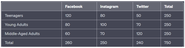
Perform a Chi-Square Test for Homogeneity to determine if the distribution of preferred social media platforms is the same across the three age groups at a significance level of 0.05.
Solution: –
Null Hypothesis (H0): The distribution of preferred social media platforms is the same across the three age groups.
Alternative Hypothesis (Ha): The distribution of preferred social media platforms is not the same across the three age groups.
Significance Level (α): 0.05
Expected Frequencies: Calculate the expected frequencies assuming homogeneity by finding the row and column totals and using these to compute the expected frequencies for each cell.
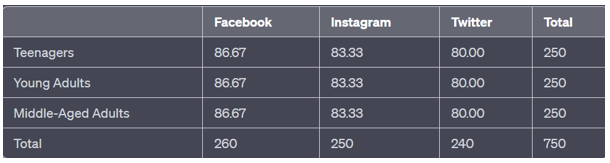
Degrees of Freedom (df): (Number of rows – 1) × (Number of columns – 1) = (3 – 1) × (3 – 1) = 4
Find Critical Value: At α = 0.05 and df = 4, the critical value from the Chi-Square distribution is approximately 9.488.
Compare Critical Value and Test Statistic: Since the test statistic (15.10) is greater than the critical value (9.488), we reject the null hypothesis.
Conclusion: There is enough evidence to conclude that the distribution of preferred social media platforms is not the same across the three age groups at a significance level of 0.05
Key Points
1. Purpose: The Chi-Square Test for Homogeneity is used to determine if the distribution of a categorical variable is the same across multiple groups or populations.
2. Categorical Data: This test is applicable when dealing with categorical data, where data points are classified into distinct categories.
3. Hypotheses: The null hypothesis (H0) states that the distributions are homogeneous (equal) across groups, while the alternative hypothesis (Ha) suggests a significant difference in distributions.
4. Expected Frequencies: Expected frequencies are calculated assuming that the distribution is the same across groups. They are used for comparison with observed frequencies.
5. Contingency Table: Data is organized into a contingency table, where rows represent groups and columns represent categories of the categorical variable.
6. Degrees of Freedom: Degrees of freedom are calculated based on the number of groups and categories, impacting the critical value and the Chi-Square statistic's interpretation.
7. Chi-Square Statistic: The Chi-Square statistic measures the difference between observed and expected frequencies. It is calculated as the sum of (observed – expected)² / expected for all cells.
8. Null Distribution: The Chi-Square statistic follows a Chi-Square distribution under the null hypothesis.
9. Critical Value: A critical value is determined based on the significance level (α) and degrees of freedom. It helps decide whether to reject the null hypothesis.
10. P-Value: The p-value is calculated based on the Chi-Square statistic and represents the probability of observing such extreme results if the null hypothesis is true.
11. Comparing P-Value and α: If p-value < α, you may reject the null hypothesis, indicating a significant difference in distributions among groups.
12. Assumptions: The Chi-Square Test for Homogeneity assumes that observations are independent and that expected frequencies are reasonably large (usually above 5).
13. Application: It is used in various fields, such as social sciences, biology, marketing, and quality control, to analyze whether different groups exhibit different categorical distributions.
14. Interpreting Results: If the null hypothesis is rejected, it implies that there is evidence of a significant difference in the distribution of the categorical variable across the groups.
15. Follow-Up Tests: If the Chi-Square Test for Homogeneity indicates a significant difference, further analysis might involve pairwise comparisons or additional statistical tests to pinpoint the specific differences.