Setting Up & Carry The Testing For Regression Model

Unit: Inference for Quantitative Data: Slopes

Chapter: Setting up & Carry the Testing for regression model

Reference: – Regression Analysis, Scatterplot, Hypothesis testing in Regression, Coefficient of determination, Residual Analysis & Diagnostics, Analyzing scatterplot & Variance, Influential Points & Outliers, Transformation, Model Comparison & Selection, Multicollinearity, ANOVA for Regression.

After studying this chapter, you should be able to:

• Regression Analysis & Scatterplot & Hypothesis Testing.
• Coefficient of Determination, Residual Analysis & Diagnostics.
• Influential Points & outliers, Model Comparison.
• Multicollinearity, ANOVA for Regression.

Regression Analysis & Scatterplot & Hypothesis Testing

Regression Analysis:

• Purpose: Regression analysis is a statistical technique used to model the relationship between a dependent variable (response) and one or more independent variables (predictors).
• Linear Relationship: Simple linear regression assumes a linear relationship between the predictor and the response variable. The goal is to find the best-fitting straight line (regression line) that minimizes the sum of squared residuals.
• Residuals: Residuals are the differences between the actual observed values and the values predicted by the regression line. The goal is to minimize the sum of squared residuals.
• Hypothesis Testing: Hypothesis tests are used to assess the significance of regression coefficients. The null hypothesis states that the coefficient is not significantly different from zero.
• Assumptions: Linear regression relies on assumptions such as linearity, constant variance (homoscedasticity), normality of residuals, and independence of errors.
• Multiple Regression: In multiple regression, two or more predictor variables are used to model the relationship with the response variable. Each predictor has its own coefficient.
• Interpreting Output: Regression output includes coefficient estimates, standard errors, p-values, and confidence intervals. These help determine the strength and significance of relationships.

Scatterplots:

• Visualization: A scatterplot is a graphical representation of individual data points on a Cartesian plane, with one variable on the x-axis and another on the y-axis.
• Relationship Assessment: Scatterplots help visualize the relationship between two variables. Patterns like linear, non-linear, or clusters can be observed.
• Correlation: The pattern of points in a scatterplot can give an indication of the correlation between the two variables. Positive correlation means points trend upwards; negative correlation means points trend downwards.
• Outliers: Outliers are data points that deviate significantly from the overall pattern in a scatterplot. They can have a strong impact on regression results.
• Strength of Relationship: The closer the points are to forming a clear linear or non-linear pattern, the stronger the relationship between the variables.
• Line of Best Fit: In a scatterplot, the line of best fit is used to visually represent the general trend of the data points. It's analogous to the regression line in regression analysis.
• Residual Analysis: Scatterplots of residuals can be used to assess the assumptions of a regression model, such as constant variance and linearity.
• Grouping: Scatterplots can include different colors or shapes to represent subgroups within the data, allowing for the examination of additional variables.
• Strength and Direction: Scatterplots provide insights into the strength and direction of relationships: positive (as one variable increases, the other also increases), negative (as one variable increases, the other decreases), or no relationship.
• Limitations: While scatterplots are informative, they might not capture complex relationships or account for the influence of other variables. Advanced statistical techniques like regression provide more rigorous analysis.

Coefficient of Determination, Residual Analysis & Diagnostics

Residual Analysis and Diagnostics:

• Residuals: Residuals are the differences between the observed values and the predicted values from the regression model. They provide insights into how well the model fits the data.
• Purpose of Residual Analysis: Residual analysis helps assess whether the assumptions of the regression model are met, including linearity, constant variance, normality, and independence of residuals.
• Residual Plots: Scatterplots of residuals against predictor variables are used to check for linearity. Scatterplots of residuals against fitted values are used to assess constant variance (homoscedasticity).
• Normality of Residuals: A histogram of residuals and a normal probability plot can help determine if residuals are approximately normally distributed.
• Influential Points: Points with high leverage or high residual values can be influential and have a significant impact on the regression model. Diagnostics identify such points.
• Outliers: Outliers are extreme data points that can affect the fit of the model. They can be identified through residual plots and influence diagnostics.
• Cook's Distance: Cook's distance measures the influence of each observation on the regression coefficients. Large Cook's distances indicate potential outliers.
• VIF (Variance Inflation Factor): VIF is used to detect multicollinearity among predictor variables. High VIF values suggest that a predictor is highly correlated with other predictors.
• Overall Fit Tests: Tests like the F-test for overall significance of the model and the lack-of-fit test help assess the appropriateness of the chosen model.
• Residual Patterns: Patterns in residual plots, such as funnel shape or non-linear trends, can indicate violations of assumptions and guide model improvements.
• Model Validation: Residual analysis is an essential step in model validation. It helps ensure that the model is reasonable and reliable for making predictions and drawing conclusions.

Standard Error & Hypothesis Testing for Slope

Standard Error:

Definition: The standard error of the slope (SE(β₁)) quantifies the average amount of variability in the estimated slope values that we would expect across different samples from the same population.

Calculation: The standard error of the slope is calculated using the formula: SE(β₁) = (estimated standard deviation of errors) / (√Σ(xi – x̄)²).

Precision: A smaller standard error indicates that the sample slope estimates are more tightly clustered around the true population slope, implying higher precision.

Sample Size: Larger sample sizes result in smaller standard errors, reflecting more accurate estimates of the population slope.

Inverse Relationship: There is an inverse relationship between the standard error of the slope and the strength of the relationship between the predictor and response variables.

Hypothesis Testing for Slope:

Null Hypothesis (H₀): In the context of hypothesis testing for the slope, the null hypothesis states that the true population slope is equal to a specified value (often zero).

Alternative Hypothesis (H₁): The alternative hypothesis complements the null hypothesis and typically states that the true population slope is not equal to the specified value.

Test Statistic (t-statistic): The t-statistic is calculated by dividing the estimated slope by its standard error. It quantifies how many standard errors the sample slope is away from the hypothesized value.

Degrees of Freedom: The degrees of freedom for the t-distribution in hypothesis testing for the slope are determined by the sample size and the number of predictor variables in the model.

Critical Values: Critical values from the t-distribution are used to establish a rejection region for the null hypothesis. The significance level (α) determines the cutoff points.

P-value: The p-value is the probability of observing a t-statistic as extreme as the one calculated from the data, assuming the null hypothesis is true. A small p-value suggests evidence against the null hypothesis.

Decision Rule: If the p-value is less than the chosen significance level (α), typically 0.05, the null hypothesis is rejected in favor of the alternative hypothesis.

Interpretation: If the null hypothesis is rejected, it indicates that there is evidence that the predictor variable has a significant effect on the response variable.

Type I and Type II Errors: Type I error occurs when the null hypothesis is incorrectly rejected, and Type II error occurs when the null hypothesis is incorrectly not rejected.

Effect Size and Practical Significance: While statistical significance is important, it's crucial to assess whether the observed effect size is practically significant and meaningful in the context of the problem.

Influential Points & Outliers & Model Comparison

Influential Points and Outliers:

• Influential Points: Influential points are data points that have a strong impact on the regression model's results, affecting parameter estimates, predictions, and overall model fit.
• Outliers: Outliers are extreme observations that deviate significantly from the rest of the data. They can be influential, but not all outliers are influential, and not all influential points are outliers.
• High Leverage: Points with high leverage have extreme values of predictor variables. They can pull the regression line towards them, affecting slope estimates.
• High Residuals: Points with high residuals (vertical distance from the regression line) can disproportionately influence the model, especially if the sample size is small.
• Influence Measures: Influence measures, such as Cook's distance and DFFITS, quantify the impact of individual observations on the regression coefficients and overall fit.
• Cook's Distance: Cook's distance measures the change in parameter estimates when a particular observation is removed from the dataset. Large Cook's distances suggest influential points.
• DFFITS: DFFITS measures the difference in predicted values when an observation is omitted. Large DFFITS values indicate influential points.
• Identifying Influential Points: Graphical tools like scatterplots of residuals or Cook's distance plots help identify influential points. A threshold value is often used to flag potential influencers.
• Impact on Results: Influential points can lead to changes in the slope, intercept, and overall fit of the regression model, potentially altering conclusions.

Model Comparison:

• Purpose of Model Comparison: Model comparison involves evaluating different regression models to determine which one provides the best fit to the data and is most appropriate for the research question.
• Nested Models: Nested models are models with varying levels of complexity, where one model is a subset of the other. Comparing nested models helps assess if added variables significantly improve the fit.
• F-Test for Model Comparison: The F-test compares the fit of the full model (with predictors) to a reduced model (without predictors) to determine if the added predictors are collectively significant.
• Adjusted R-squared: Adjusted penalizes the inclusion of unnecessary predictors. It helps compare models and choose the one that balances model complexity with explanatory power.
• AIC and BIC: Information criteria like AIC (Akaike Information Criterion) and BIC (Bayesian Information Criterion) provide quantitative measures for comparing models. Lower values indicate better fit.
• Overfitting and Underfitting: Overfitting occurs when a model is too complex and fits noise in the data. Underfitting occurs when a model is too simple to capture the underlying relationship. Model comparison helps strike a balance.
• Cross-Validation: Cross-validation techniques, such as k-fold cross-validation, help assess how well a model generalizes to new data. It aids in comparing different models' predictive performance.
• Practical Considerations: When comparing models, factors like interpretability, domain knowledge, and the research question should also be taken into account, not just statistical measures.
• Occam's Razor: Model comparison often aligns with Occam's Razor principle: preferring simpler models that explain the data well without unnecessary complexity.

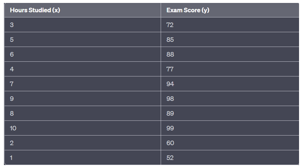
Example: Predicting Exam Scores

Suppose you are a statistics student interested in understanding how the number of hours students spend studying correlates with their exam scores. You collect data from a random sample of 10 students, recording the number of hours they studied and their corresponding exam scores:

Solution: – Step 1: Calculate the P-value

Using the test statistic, calculate the p-value associated with the t-test. This p-value represents the probability of observing a t-statistic as extreme as the one calculated, assuming the null hypothesis is true.

Step 2: Make a Decision

Using the calculated p-value and a chosen significance level (α), compare the p-value to α to make a decision about the null hypothesis. If the p-value is less than α, you reject the null hypothesis; otherwise, you fail to reject the null hypothesis.

Solution:

Let's assume we calculate the test statistic as 2.31 and the corresponding p-value is 0.0420.042. If we choose a significance level of =0.05, then:

• Decision: Since 0.042<0.050.042<0.05, we reject the null hypothesis.

Conclusion:

Based on the analysis, we have evidence to conclude that there is a statistically significant linear relationship between the number of hours studied and exam scores. In other words, the number of hours studied has a significant impact on exam scores for the given sample of students.

Key Points

• Hypotheses: Start by stating the null hypothesis and alternative hypothesis (Ha​) about the relationship between the predictor and response variables.
• Data Collection: Gather a sample of data pairs that includes the predictor and response values.
• Regression Line: Use software to find the regression line that best fits the data, which shows the overall trend.
• Residuals: Calculate the differences between the actual response values and the predicted values from the regression line.
• Assumptions Check: Verify key assumptions like linearity (points form a roughly straight line), constant variance (residuals spread evenly), normality of residuals, and independence of errors.
• Test Statistic: Compute a statistic that helps you understand if the predictor is significantly related to the response.
• Degrees of Freedom: Determine how many degrees of freedom are associated with the test statistic.
• P-value: Find the p-value, which tells you the probability of observing the results if there is no real relationship between the variables.
• Significance Level (α): Choose a significance level that determines how strong the evidence needs to be to reject the null hypothesis.
• Decision: Compare the p-value to the significance level to decide whether to reject the null hypothesis or not.
• Conclusion: Based on the decision, draw a conclusion about whether there is a statistically significant relationship.
• Coefficient Interpretation: If the relationship is significant, interpret the slope coefficient in terms of the variables' connection.
• Confidence Interval: Calculate a range of values where you're fairly certain the actual slope lies.
• Coefficient of Determination: Assess how well the regression line fits the data by looking at the value, which tells you the proportion of variability explained.
• Assumptions Review: After testing, revisit the assumptions to make sure your findings are valid and reliable.