Rates, Linearity & Approximation

Unit: Contextual Application of Differentiation

Chapter: Rates, Linearity & Approximation

Reference: – Average rate of change, Slope of a line, Tangent line, Derivatives, Linear approximation, Linear functions & Graphs, Piecewise linear functions, Indeterminate form, Continuity of a function, Taylor series, Maclaurin series, Linear regression.

After studying this chapter, you should be able to:

• Introduction, Tangent lines & Derivatives.
• Mean Value Theorem & Linear Approximation.
• Related rates & Motion in a plane.

Introduction, Tangent Lines & Derivatives

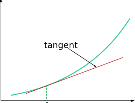
1. Tangent Lines:

• A tangent line is a line that touches a curve at a specific point, without crossing or intersecting it. In calculus, the tangent line to a curve at a given point represents the instantaneous rate of change or slope of the curve at that point.

• The tangent line provides a local linear approximation to the curve near that point.

1. Derivatives:

• Derivatives are a fundamental concept in calculus and are used to describe the rate at which a function changes. The derivative of a function f(x) at a specific point represents the slope of the tangent line to the graph of the function at that point.

• The derivative of a function f(x) is denoted as f'(x) or dy/dx. It can be interpreted as the limit of the average rate of change of the function as the interval approaches zero.

•  The derivative measures how the function behaves locally around a given point.                          

Mean Value Theorem & Linear Approximation:

Mean Value Theorem:

• The Mean Value Theorem (MVT) is a fundamental result in calculus that connects the average rate of change of a function with its instantaneous rate of change.

• According to the MVT, if a function f(x) is continuous on the closed interval [a, b] and differentiable on the open interval (a, b), then there exists at least one point c in (a, b) where the instantaneous rate of change (derivative) of the function is equal to the average rate of change of the function over the interval [a, b].

• Geometrically, the MVT states that there exists a tangent line parallel to the secant line connecting the endpoints of the interval. The slope of this tangent line is equal to the average rate of change of the function.

• The MVT is often used to prove important results in calculus, such as the existence of critical points and the behavior of functions.

• The MVT is a special case of Rolle's Theorem, which states that if a function is continuous on [a, b] and differentiable on (a, b) with f(a) = f(b), then there exists at least one point c in (a, b) where the derivative is zero.

Linear Approximation:

• Linear approximation is a technique used to approximate the value of a function near a specific point by using a tangent line to the curve at that point.

• The tangent line provides a good approximation of the function's behavior in the vicinity of the point of tangency.

• The equation of the tangent line can be obtained by finding the slope of the tangent (which is the derivative of the function at the point) and using the point-slope form of a line.

• Linear approximation is based on the idea that for small enough intervals, a function can be approximated by a linear function (tangent line) with a negligible error.

• Linear approximation is useful for estimating function values, calculating small changes or differentials, and simplifying more complex functions for analysis.

Velocity, Acceleration & Optimization: –

• Velocity Functions: Nested functions refer to functions that are composed together in a sequence, where the output of one function becomes the input of another.

• Function Composition: When functions are nested, the output of the inner function serves as the input to the outer function. This composition allows for more complex transformations of variables.

• Acceleration Function: The inner function refers to the function that is placed inside another function. It typically takes an independent variable as its input and produces an output.

• Outer Function: The outer function refers to the function that contains the inner function. It takes the output of the inner function as its input and produces the final output of the nested function.

• Variables in Nested Functions: When dealing with nested functions, it's important to consider the variables involved at different levels.

• Independent Variable: The independent variable is typically associated with the innermost function. It represents the input to the nested function and is usually denoted as x.

• Intermediate Variables: In a nested function, there can be intermediate variables between the inner and outer functions. These variables are generated during the evaluation of the inner function and serve as inputs to the outer function.

• Dependent Variable: The dependent variable represents the final output of the nested function and is typically denoted as y.

• Differentiation of Nested Functions: When differentiating a nested function, the chain rule is applied iteratively. The derivative of the outer function for its input is multiplied by the derivative of the inner function for its input, which can involve additional intermediate variables.

• Order of Evaluation: When differentiating a nested function, it's important to evaluate the derivatives in the correct order, starting from the innermost function and moving outward.

                                          (Linearity Graph)

Related Rates & Motion in a Plane: –

Related Rates:

• Related Rates problems involve analyzing the rates at which different variables are changing over time and finding the relationship between their rates of change.

• These problems typically involve multiple variables that are related through an equation or geometric relationship.

• The key to solving related rates problems is to differentiate the given equation or relationship for a time, treating the variables as functions of time.

• The chain rule is often used to differentiate composite functions in related rate problems.

• Once the equation is differentiated, the rates of change of the variables can be plugged in, and the problem can be solved for the desired rate of change.

Motion in a Plane:

• Motion in a plane refers to the study of objects moving in two dimensions, typically described by parametric equations or vector-valued functions.

• Parametric equations represent the x and y coordinates of a point on a curve as functions of an independent parameter, often time.

• Vector-valued functions describe the position of an object at a given time using vector notation, with separate components for x and y coordinates.

• Motion in a plane problem involves analyzing velocity, acceleration, displacement, and other properties of objects in motion.

• Projectile motion is a common example of motion in a plane, where objects are launched into the air and follows a curved trajectory under the influence of gravity.

Example: – Find the general solution of the differential equation.

Solution:

Before starting to solve the differential equation, we should know the type of differential equation.

This is the linear type differential equation,

y dx – (x + 2y²)dy = 0

It is of the form  dx/dy + Rx = S where R and S are either constants or functions of y.

To solve these types of equations, we need first to find the integrating factor, which is =  eR dy, and multiply both sides of the general form of the equation and, after that integrate the whole equation.

First, convert the given equation into general-form equation,

R =  -1/y  and S = 2y

Now find the I.F. =

Multiplying both sides by I.F. we get,

Integrating both sides concerning y, we get,

Key Points

• Rates involve measuring the change in one quantity concerning another, often represented as a ratio of the two quantities.

• The average rate of change is determined by calculating the difference in the values of a quantity over a given interval.

• The instantaneous rate of change represents the rate of change at a specific point and is found by taking the derivative of a function.

• Rates are essential in understanding the behavior of functions, such as determining increasing or decreasing intervals.

• Linearity refers to the property of a function that follows a straight line, indicating a constant rate of change.

• Linear functions can be represented by the equation y = mx + b, where m is the slope and b is the y-intercept.

• Linearity is associated with proportional relationships and constant rates.

• The concept of linearity extends to the derivative of a function, where a linear function has a constant derivative.

• Approximation involves estimating the value of a quantity based on limited information or simplifying a complex function.

• The linear approximation uses tangent lines to approximate the behavior of a function near a specific point.

• The tangent line provides a close approximation to the function's value and slope in the vicinity of the point of tangency.

• Approximation techniques are valuable for making calculations more manageable, estimating changes, and providing simplified models for analysis.