Unit: Contextual Application of Differentiation
Chapter: Generalizing Motion to rate of Change
Reference: – Polar Coordinates, 3- Dimensional motion, Circular motion, Curvature, Projectile Motion, Chain rule, Tangent & Normal Vectors, Fundamental Theorem, Notations & its applications.
After studying this chapter, you should be able to:
- Average & Instantaneous rate of change.
- Tangent line, Derivatives & Differentiation rule.
- Notations & Application of Differentiation.
Introduction & Rate of Change
- Average Rate of Change: The average rate of change of a function over an interval is determined by finding the slope of the secant line connecting two points on the graph of the function. It measures how the output of the function changes on average for a given change in the input. The formula for the average rate of change between two points (x₁, f(x₁)) and (x₂, f(x₂)) is given by:
- Average Rate of Change = (f(x₂) – f(x₁)) / (x₂ – x₁)
This concept is often used to approximate instantaneous rates of change when the interval becomes very small.
- Instantaneous Rate of Change: The instantaneous rate of change refers to the rate at which a function is changing at a specific point. It provides a precise measure of how the output of a function is changing concerning the input at that particular point. The instantaneous rate of change is represented by the derivative of the function at that point.
- To find the instantaneous rate of change, we take the limit of the average rate of change as the interval between the two points approaches zero. Mathematically, this is expressed as:
- Instantaneous Rate of Change = lim (x→a) (f(x) – f(a)) / (x – a)
- where 'a' is the specific point at which we want to find the instantaneous rate of change.
Tangent Lines, Derivatives & Differentiation Rule:
To obtain the differential equation, we follow the following steps:-
Step 1: Differentiate the given function w.r.t from the independent variable present in the equation.
Step 2: Keep differentiating times in such a way that (n + 1) equations are obtained.
Step 3: Using the (n + 1) equations obtained, eliminate the constants (c1, c2, … cn).
Procedure to form a differential equation that will represent a given family of curves
(a) If the given family F1 of curves depends on only one parameter, then it is represented by an equation of the form
F1 (x, y, a) = 0 … (1)
For example, the family of parabolas y2 = ax can be represented by an equation of form f (x, y, a) : y2 = ax.
Differentiating equation (1) with respect to x, we get an equation involving y’, y, x, and a, i.e.,
g (x, y, y’, a) = 0 … (2)
The required differential equation is then obtained by eliminating a from equations (1) and (2) as
F (x, y, y’) = 0 … (3)
(b) If the given family F2 of curves depends on the parameters a, b (say) then it is represented by an equation of the form
F2 (x, y, a, b) = 0 … (4)
Differentiating equation (4) with respect to x, we get an equation involving y’, x, y, a, b, i.e.,
g (x, y, y’, a, b) = 0 … (5)
But it is not possible to eliminate two parameters a and b from the two equations, so, we need a third equation. This equation is obtained by differentiating equation (5), with respect to x, to obtain a relation of the form
h (x, y, y’, y’’, a, b) = 0 … (6)
The required differential equation is then obtained by eliminating a and b from equations (4), (5), and (6) as
F (x, y, y’, y’’) = 0 … (7)
Note: The order of a differential equation representing a family of curves is the same as the number of arbitrary constants present in the equation corresponding to the family of curves.
Example:
Form the differential equation of the family of curves represented by y2 = (x – c)3.
Solution:
y2 = (x – c)3
On differentiating the above equation for x we get
![]()
![]()
Putting the value of (x – c) in the given equation, we get,
On squaring, both sides we get,
![]()
![]()
![]()
Hence,
![]()
is the differential equation which represents the family of curves y2 = (x – c)3.
Example:
Form the differential equation corresponding to y = emx by eliminating m.
Solution:
Given equation, y = emx
On differentiating the above equation with respect to x we get
![]()
But y = emx
![]()
Now we have, y = emx
Applying log on both sides, we get,
log y = mx
which gives
![]()
So, putting this value of m in dydx![]() =my we get
=my we get
![]()
![]()
Hence,
![]()
is the differential equation corresponding to y = emx.
Notations & Applications of Differentiation: –
- Integration of g(y) dy: Integrate the left side of the separated equation, which involves finding the antiderivative of the function g(y) concerning y.
- Integration of f(x) dx: Integrate the right side of the separated equation, which involves finding the antiderivative of the function f(x) concerning x.
- The constant of integration: After integrating both sides, you will obtain an equation of form F(y) = G(x) + C, where F(y) and G(x) are the antiderivatives of g(y) and f(x), respectively, and C is the constant of integration.
- Evaluate the constant of integration: If initial conditions are provided, you can use them to determine the value of the constant of integration (C).
- Simplification and additional steps: After evaluating the constant of integration, you may need to simplify the equation or perform additional algebraic manipulations to express the solution in a more suitable form.
- Check for validity: Finally, it is important to check the validity of the obtained solution by differentiating it and substituting it back into the original differential equation.
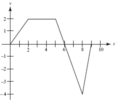
(Generalizing motion graph)
Particular Solution & Applications: –
- Applications: Separable differential equations find applications in various fields of mathematics and science. Some common applications include population dynamics, radioactive decay, chemical reactions, growth models, fluid flow, and electrical circuits.
- General Solution: When solving a separable differential equation, the goal is to find the general solution. The general solution represents a family of solutions that satisfy the differential equation. It contains a constant integration that allows for different specific solutions within the family.
- Initial Conditions: To obtain a specific solution from the general solution, we need to apply initial conditions. These conditions specify the value(s) of the dependent variable(s) at a particular point or time.
- Existence and Uniqueness: It is important to note that not all separable differential equations have unique solutions. The existence and uniqueness of solutions depend on certain conditions.
- Singular Solutions: In some cases, a separable differential equation may have singular solutions. These solutions arise when the constant of integration takes a particular value.
- Phase Diagrams: Separable differential equations can be represented graphically using phase diagrams. Phase diagrams illustrate the behavior of the solutions over time or for different initial conditions.
- Numerical Methods: In situations where analytical solutions are not readily obtainable, numerical methods such as Euler's method, Runge-Kutta methods, or finite difference methods can be employed to approximate the solutions of separable differential equations.
Key Points
- Generalizing motion to rate of change in AP Calculus involves studying how the rate of change of a function relates to motion.
- The average rate of change measures the average rate at which a quantity changes over an interval.
- The instantaneous rate of change determines the rate of change of a function at a specific point.
- The derivative of a function represents the instantaneous rate of change at each point and provides the slope of the tangent line.
- Differentiation rules, such as the power rule and chain rule, are used to calculate derivatives efficiently.
- The derivative notation includes Leibniz notation (dy/dx), prime notation (f'), and the rate of change notation (df/dx).
- Tangent lines to the graph of a function represent the instantaneous rate of change at a specific point.
- The derivative can be interpreted as the velocity when dealing with position-time functions.
- Acceleration can be determined by taking the derivative of velocity or the second derivative of position.
- Related rates problems involve finding the rates at which quantities change when they are related through an equation.
- Implicit differentiation is often used for differential equations that cannot be solved explicitly for a variable.
- Generalizing motion to rate of change allows for analyzing and solving problems involving rates of change in various contexts, such as physics and economics.