Unit: Differential Equation
Chapter: Exponential Growth & Decay
Reference: – First & Second derivative, Higher order derivative, Notations, Power rule, Product rule, Quotient rule, Chain rule, Differentiation of higher order, Exponential function, Logarithmic & Polynomial Functions, Concavity, Inflection point & Applications.
After studying this chapter, you should be able to:
- Simple Growth & Decay Model.
- Discrete Compounding & Solution Techniques.
- Half-Life, Doubling Time & Applications.
Introduction to Simple Growth & Decay Model
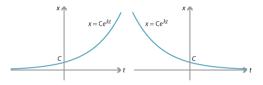
- Differential Equation Form: Simple growth and decay models can be described using a basic form of the differential equation, known as the exponential growth or decay equation. The equation takes the form dy/dt = ky, where y represents the quantity being modeled, t is time, and k is a constant representing the growth or decay rate.
- Exponential Growth: In the case of exponential growth, the growth rate k is positive, leading to an increasing quantity over time. The rate of growth is proportional to the current quantity, resulting in rapid growth as the quantity becomes larger. Examples of exponential growth include population growth and the spread of infections in an epidemic.
- Exponential Decay: Exponential decay occurs when the growth rate k is negative, resulting in a decreasing quantity over time. Similar to exponential growth, the rate of decay is proportional to the current quantity, leading to rapid decay as the quantity becomes smaller. Radioactive decay and the decay of pollutants in the environment are examples of exponential decay.
- The Law of Natural Growth and Decay: Simple growth and decay models are based on the Law of Natural Growth and Decay, which states that the rate of change of a quantity is directly proportional to the quantity itself. This law provides the foundation for the exponential growth and decay equations.
- Solution of the Differential Equation: The solution to the exponential growth or decay differential equation is given by y = y0 * e^(kt), where y0 is the initial quantity at time t=0, and e is Euler's number, a mathematical constant approximately equal to 2.71828. The exponential term captures the growth or decay behavior over time.
- Half-Life: In exponential decay models, the concept of half-life is important. The half-life is the time it takes for a quantity to reduce to half its initial value. It is determined by the decay constant k, where half-life = ln(2)/|k|. The shorter the half-life, the faster the decay rate.
- Doubling Time: Conversely, in exponential growth models, the doubling time is the time it takes for a quantity to double its initial value. It can be determined by doubling time = ln(2)/k. The shorter the doubling time, the faster the growth rate.
(Exponential Growth & Decay)
Discrete Compounding & Solution Technique:
- Separation of Variables: One common technique is the separation of variables. This method involves rearranging the differential equation by separating the variables, typically placing all terms involving the dependent variable on one side and all terms involving the independent variable on the other side.
- Integrating Factors: Another approach is using integrating factors. This technique involves multiplying the entire differential equation by a suitable integrating factor that transforms the equation into an exact differential equation. This allows for direct integration and obtaining the solution.
- Exponential Function Method: Since exponential growth and decay equations have exponential terms, an effective method is to assume a solution of the form y = Ce^(kt), where C is a constant and k is the growth or decay rate. Plugging this assumed solution into the differential equation and solving for k and C will yield the specific solution.
- Initial Value Problems: For exponential growth and decay models, it is common to have initial conditions or known values at a specific time. These initial value problems can be solved by substituting the given initial conditions into the general solution obtained through the techniques mentioned above. This allows for determining the specific constants and obtaining a unique solution.
- Half-Life and Doubling Time: When dealing with exponential decay or growth models, it is often useful to calculate the half-life or doubling time. The half-life represents the time it takes for the quantity to decrease by half, while the doubling time is the time it takes for the quantity to double. These values can be determined using logarithmic properties and are related to the growth or decay rate.
- Numerical Methods: In some cases, it may be challenging to obtain an analytical solution to exponential growth and decay equations. In such situations, numerical methods can be employed. Numerical methods, such as Euler's method or Runge-Kutta method, approximate the solution by discretizing the differential equation and iteratively calculating the values at different time points.
- Graphical Analysis: Another way to analyze exponential growth and decay is through graphical methods. Plotting the solutions on a graph can provide insights into the behavior of the quantity over time. It allows for visualizing the growth or decay rate, equilibrium points, and the impact of different parameters.
Boundary Value & Applications: –
- Integration of g(y) dy: Integrate the left side of the separated equation, which involves finding the antiderivative of the function g(y) for y.
- Integration of f(x) dx: Integrate the right side of the separated equation, which involves finding the antiderivative of the function f(x) for x.
- A constant of integration: After integrating both sides, you will obtain an equation of form F(y) = G(x) + C, where F(y) and G(x) are the antiderivatives of g(y) and f(x), respectively, and C is the constant of integration.
- Evaluate the constant of integration: If initial conditions are provided, you can use them to determine the value of the constant of integration (C).
- Simplification and additional steps: After evaluating the constant of integration, you may need to simplify the equation or perform additional algebraic manipulations to express the solution in a more suitable form.
- Check for validity: Finally, it is important to check the validity of the obtained solution by differentiating it and substituting it back into the original differential equation.
(Boundary Value)
Half-Life Doubling time & Applications: –
- Half-life refers to the time it takes for a quantity to reduce to half of its initial value in an exponential decay process. It is denoted by the symbol "t½". The half-life is a characteristic property of the decay process and remains constant regardless of the initial quantity.
- The half-life can be determined using the decay constant (k) in the exponential decay equation. The formula for calculating the half-life is given by t½ = ln(2)/k, where ln denotes the natural logarithm. The shorter the half-life, the faster the decay rate.
Doubling Time
- Doubling time refers to the time it takes for a quantity to double its initial value in an exponential growth process. It is denoted by the symbol "T₂". The doubling time is inversely proportional to the growth rate (k) in the exponential growth equation.
- The formula for calculating the doubling time is given by T₂ = ln(2)/k, where ln denotes the natural logarithm. The shorter the doubling time, the faster the growth rate.
Example: -Verify that the function y = a cos x + b sin x, where, a, b Î R is a solution of the differential equation ![]()
Solution: y = a cos x + b sin x … (1)
Differentiating both sides of equation (1) for x, we get
dy/dx = – a sinx + b cos x
![]() = – a cos x – b sinx = -(a cos x + b sin x) = -y
= – a cos x – b sinx = -(a cos x + b sin x) = -y
![]() + y = 1
+ y = 1
Hence proved.
Key Points
- Differential Equation: Exponential growth and decay are modeled using differential equations of the form dy/dt = ky, where y represents the quantity, t is time, and k is the growth or decay rate constant.
- Exponential Growth: In exponential growth, the growth rate k is positive, resulting in a quantity that increases rapidly over time. The rate of growth is proportional to the current quantity.
- Exponential Decay: Exponential decay occurs when the growth rate k is negative, leading to a quantity that decreases rapidly over time. The rate of decay is proportional to the current quantity.
- Exponential Function: Exponential growth and decay equations are typically solved using exponential functions of the form y = C * e^(kt), where C is the initial quantity and e is Euler's number, approximately 2.71828.
- Half-Life: The half-life is the time it takes for a quantity to reduce to half its initial value in an exponential decay process. It is determined by the decay constant k, where half-life = ln(2)/|k|. A shorter half-life indicates faster decay.
- Doubling Time: Doubling time refers to the time it takes for a quantity to double its initial value in an exponential growth process. Doubling time = ln(2)/k. A shorter doubling time indicates faster growth.
- Initial Value Problems: Exponential growth and decay models often involve initial conditions, where the quantity is known at a specific time. These initial value problems help determine the specific constants and obtain a unique solution.
- Solution Techniques: Various techniques can be used to solve exponential growth and decay differential equations, such as the separation of variables, integrating factors, or assuming an exponential solution form.
- Stability and Equilibrium: Exponential growth and decay models have equilibrium solutions, where the quantity remains constant over time. The stability of the equilibrium is determined by the sign of the growth or decay rate constant.
- Applications: Exponential growth and decay models have numerous applications, including population dynamics, radioactive decay, financial investments, drug clearance, environmental studies, and biological processes.