Unit: Differential Equation

Chapter: General & Particular Solution

Reference: – Polar Coordinates, 3- Dimensional motion, Circular motion, Curvature, Projectile Motion, Chain rule, Tangent & Normal Vectors, Fundamental Theorem, Notations & its applications.

After studying this chapter, you should be able to:

• First Order & Second Order Differential Equation.
• General solution & Particular solution.
• Boundary Value & Applications.

Introduction & First Order Equation

• Separable Equations: These are equations that can be separated into two separate functions, one involving only the dependent variable and the other involving only the independent variable. By integrating both sides of the equation separately, you can find the general solution.

• Linear Equations: Linear first-order differential equations have the form dy/dx + p(x)y = q(x), where p(x) and q(x) are given functions. These equations can be solved using an integrating factor, which involves multiplying both sides of the equation by an appropriate function to make it integrable.

• Exact Equations: An exact differential equation can be written in the form M(x, y)dx + N(x, y)dy = 0, where M and N are functions of x and y, and the equation satisfies the condition ∂M/∂y = ∂N/∂x. Solving exact equations involves finding a potential function such that its partial derivatives for x and y match the coefficients of dx and dy in the given equation.

• Homogeneous Equations: Homogeneous first-order differential equations are of the form dy/dx = f(x, y)/g(x, y), where f(x, y) and g(x, y) are homogeneous functions of the same degree. Homogeneous equations can be solved using a substitution to reduce the equation to a separable form.

• Bernoulli Equations: Bernoulli differential equations have the form dy/dx + p(x)y = q(x)yⁿ, where p(x), q(x), and n are given functions or constants. By applying a suitable substitution, these equations can be transformed into linear equations, making them solvable.

• Integrating Factors: Integrating factors are used to solve linear differential equations by multiplying both sides of the equation by a suitable function to make it integrable. The integrating factor is determined by the coefficient function of the dependent variable.

General Solution & Particular Solution:

To obtain the differential equation, we follow the following steps:-

Step 1: Differentiate the given function w.r.t from the independent variable present in the equation.

Step 2: Keep differentiating times in such a way that (n + 1) equations are obtained.

Step 3: Using the (n + 1) equations obtained, eliminate the constants (c₁, c₂, … c_n).

Procedure to form a differential equation that will represent a given family of curves

(a)    If the given family F₁ of curves depends on only one parameter, then it is represented by an equation of the form

         F₁ (x, y, a) = 0                                                       … (1)

For example, the family of parabolas y² = ax can be represented by an equation of form f (x, y, a) : y² = ax.

Differentiating equation (1) with respect to x, we get an equation involving y’, y, x, and a, i.e.,

g (x, y, y’, a) = 0                                            … (2)

The required differential equation is then obtained by eliminating a from equations (1) and (2) as

F (x, y, y’) = 0                                                        … (3)

(b)    If the given family F₂ of curves depends on the parameters a, b (say) then it is represented by an equation of the form

F₂ (x, y, a, b) = 0                                                    … (4)

Differentiating equation (4) with respect to x, we get an equation involving y’, x, y, a, b, i.e.,

g (x, y, y’, a, b) = 0                                                 … (5)

But it is not possible to eliminate two parameters a and b from the two equations, so, we need a third equation. This equation is obtained by differentiating equation (5), for x, to obtain a relation of the form

h (x, y, y’, y’’, a, b) = 0                                            … (6)

The required differential equation is then obtained by eliminating a and b from equations (4), (5), and (6) as

F (x, y, y’, y’’) = 0                                                   … (7)

Note: The order of a differential equation representing a family of curves is the same as the number of arbitrary constants present in the equation corresponding to the family of curves.

Example:

Form the differential equation of the family of curves represented by y² = (x – c)³.

Solution:

y² = (x – c)³

On differentiating the above equation for x we get

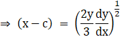
Putting the value of (x – c) in the given equation, we get,

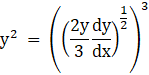
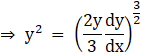
On squaring, both sides we get,

Hence,

 is the differential equation which represents the family of curves y² = (x – c)³.

Example:

Form the differential equation corresponding to y = e^mx by eliminating m.

Solution:

Given equation, y = e^mx

On differentiating the above equation for x we get

But y = e^mx

Now we have, y = e^mx

Applying log on both sides, we get,

log y = mx

which gives

So, putting this value of m in  dy/dx  =my   we get

Hence,

is the differential equation corresponding to y = e^mx.

Boundary Value & Applications: –

• Integration of g(y) dy: Integrate the left side of the separated equation, which involves finding the antiderivative of the function g(y) for y.

• Integration of f(x) dx: Integrate the right side of the separated equation, which involves finding the antiderivative of the function f(x) for x.

• A constant of integration: After integrating both sides, you will obtain an equation of form F(y) = G(x) + C, where F(y) and G(x) are the antiderivatives of g(y) and f(x), respectively, and C is the constant of integration.

• Evaluate the constant of integration: If initial conditions are provided, you can use them to determine the value of the constant of integration (C).

• Simplification and additional steps: After evaluating the constant of integration, you may need to simplify the equation or perform additional algebraic manipulations to express the solution in a more suitable form.

• Check for validity: Finally, it is important to check the validity of the obtained solution by differentiating it and substituting it back into the original differential equation.

                                         (Boundary Value)

Particular Solution & Applications: –

• Applications: Separable differential equations find applications in various fields of mathematics and science. Some common applications include population dynamics, radioactive decay, chemical reactions, growth models, fluid flow, and electrical circuits.

• General Solution: When solving a separable differential equation, the goal is to find the general solution. The general solution represents a family of solutions that satisfy the differential equation. It contains a constant integration that allows for different specific solutions within the family.

• Initial Conditions: To obtain a specific solution from the general solution, we need to apply initial conditions. These conditions specify the value(s) of the dependent variable(s) at a particular point or time.

• Existence and Uniqueness: It is important to note that not all separable differential equations have unique solutions. The existence and uniqueness of solutions depend on certain conditions.

• Singular Solutions: In some cases, a separable differential equation may have singular solutions. These solutions arise when the constant of integration takes a particular value.

• Phase Diagrams: Separable differential equations can be represented graphically using phase diagrams. Phase diagrams illustrate the behavior of the solutions over time or for different initial conditions.

• Numerical Methods: In situations where analytical solutions are not readily obtainable, numerical methods such as Euler's method, Runge-Kutta methods, or finite difference methods can be employed to approximate the solutions of separable differential equations.

Key Points

• General solution: The general solution of a differential equation represents a family of solutions that satisfy the equation. It contains arbitrary constants that can be determined by applying initial or boundary conditions.

• Particular solution: A particular solution is a specific solution that satisfies both the differential equation and any given initial or boundary conditions. It is obtained by assigning specific values to the arbitrary constants in the general solution.

• Arbitrary constants: The general solution of a differential equation contains arbitrary constants. These constants represent degrees of freedom and allow for a variety of possible solutions.

• Initial conditions: To find a particular solution, initial conditions are often provided. These conditions specify the values of the dependent variable and its derivatives at a particular point in the domain of the equation.

• Boundary conditions: For differential equations defined on a certain interval, boundary conditions are provided. These conditions specify the values of the dependent variable or its derivatives at the endpoints of the interval.

• The uniqueness of particular solutions: A well-posed differential equation with appropriate initial or boundary conditions has a unique particular solution. This means that there is only one solution that satisfies the given conditions.

• Superposition principle: The superposition principle states that if two or more solutions satisfy a linear homogeneous differential equation, then any linear combination of these solutions is also a solution.

• Non-homogeneous equations: Non -Homogeneous differential equations have terms that depend on the independent variable. To find the particular solution, additional techniques like variation of parameters or the method of undetermined coefficients may be used.

• Homogeneous equations: Homogeneous differential equations have no terms that depend on the independent variable. The general solution of a homogeneous equation is obtained by setting the right-hand side of the equation to zero.

• Existence of solutions: The existence of solutions for a differential equation depends on various factors, including the form of the equation, the domain of the equation, and the given conditions. Well-posed problems with appropriate conditions typically have unique solutions.