Position Of Particle Moving In Plane

Unit: Parametric Equations, Polar Coordinates & Vector-Valued Function

Chapter: Position of Particles Moving in plane

Reference: – Position vectors, Velocity vectors, Acceleration vectors, Scalar & Vector functions, Tangent vector, Tangent lines, Normal vector, Normal lines, Curvature & Arc length of a curve, Projectile Motion & Relative motion, Polar equations, Application of Vector calculus

After studying this chapter, you should be able to:

• Introduction to Position vectors & Velocity vectors.
• Parametric & Polar equations.
• Projectile & Relative motion.
• Application of vector calculus to particle motion.

Introduction to Position & Velocity Vectors

• Position Vector: A position vector is a vector that describes the location of a point in space relative to a reference point or origin.

• Magnitude: The magnitude of a position vector represents the distance between the reference point and the point in space.

• Direction: The direction of a position vector is determined by the angle it makes with a reference axis or by its components in a coordinate system.

• Velocity Vector: A velocity vector is a vector that describes the rate of change of position of an object for time.

• Tangent Vector: The velocity vector at a specific point on a curve is tangent to the curve at that point.

• Magnitude: The magnitude of a velocity vector represents the speed of an object, which is the rate at which it covers distance.

• Direction: The direction of a velocity vector represents the direction in which the object is moving.

• Derivative: The velocity vector is obtained by taking the derivative of the position vector for time.

• Instantaneous Velocity: The velocity vector at a specific instant in time is known as the instantaneous velocity.

• Average Velocity: The average velocity vector is the displacement vector divided by the time interval over which the displacement occurs.

• Unit Vectors: Position and velocity vectors are often expressed using unit vectors, such as the i, j, and k vectors in Cartesian coordinate systems.

• Components: Position and velocity vectors can be broken down into their components along the coordinate axes to simplify calculations.

• Vector Addition: Position and velocity vectors can be added or subtracted using vector addition or subtraction rules.

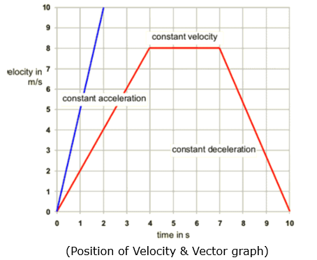
• Graphical Representation: Position and velocity vectors can be graphically represented using arrows, where the length represents magnitude, and the direction represents direction.

Introduction to Vector-Valued Functions: –

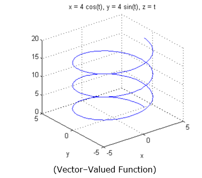
1. Vector-valued functions are functions that map a real number (usually denoted as t) to a vector in two or three-dimensional space.

1. Vector-valued functions are often used to describe the motion of objects in space or the path of a particle.

1. The components of a vector-valued function represent the coordinates of a point in space as functions of t.

1. The derivative of a vector-valued function represents the rate of change of the position vector for t, often interpreted as the velocity vector.

1. The derivative of a vector-valued function is found by differentiating each component of the function separately.

1. The chain rule is used to find the derivatives of vector-valued functions by applying the derivative to each component and combining the results.

1. The second derivative of a vector-valued function represents the rate of change of the velocity vector and is interpreted as the acceleration vector.

1. Tangent vectors to a vector-valued function can be found by evaluating the derivative at a specific value of t, representing the direction of motion at that point.

1. The magnitude of the derivative of a vector-valued function represents the speed or magnitude of the velocity vector.

1. The arc length of a vector-valued function can be calculated using integrals and a specific formula that takes into account the derivative of the vector-valued function.

1. Vector-valued functions can be used to model various real-world scenarios, such as the trajectory of a projectile, the motion of a particle, or the path of a moving object.

1. Vector-valued functions are also essential in studying topics such as curves in space, motion in three dimensions, and the fundamental principles of calculus in higher dimensions.

Parametric & Polar Equation

Parametric Equations:

• Parametric Equations: Parametric equations describe the position of a particle in terms of one or more independent parameters, typically denoted as t.

• Parameter: The parameter t represents time or any other independent variable that determines the position of the particle.

• Coordinate Functions: Parametric equations consist of coordinate functions that define the x and y coordinates of the particle as functions of the parameter.

• Independence: Parametric equations provide a way to describe paths that are not easily represented by a single equation, such as curves and complex motions.

• Graphical Representation: The graph of parametric equations often yields a curve in the plane, showing how the x and y coordinate change as the parameter varies.

• Tangent Line: The tangent line to a curve defined by parametric equations can be found by taking the derivatives of the coordinate functions for the parameter.

• Arc Length: Parametric equations allow for the calculation of arc length, which represents the length of the curve traveled by the particle.

• Velocity Vector: The velocity vector of a particle moving along a parametric curve is obtained by differentiating the coordinate functions for the parameter.

• Acceleration Vector: The acceleration vector is obtained by taking the derivative of the velocity vector for the parameter.

Polar Equations:

• Polar Coordinates: Polar equations describe the position of a particle in terms of a distance from a fixed point (pole) and an angle from a fixed reference line (usually the positive x-axis).

• Polar Equation Form: Polar equations are typically expressed in the form r = f(θ), where r represents the distance and θ represents the angle.

• Graphical Representation: Polar equations generate curves in polar coordinates, representing various shapes such as circles, ellipses, spirals, and more.

• Symmetry: Polar equations often exhibit symmetry for the pole, the origin, or certain angles.

• Tangent Line: The tangent line to a polar curve can be found by taking the derivative of the polar equation and applying trigonometric identities.

• Area Enclosed: Polar equations allow for the calculation of the area enclosed by a polar curve using integration techniques.

Projectile & Relative Motion

Projectile Motion:

• Projectile: A projectile is an object that is launched into the air and moves along a curved path under the influence of gravity.

• Trajectory: The path followed by a projectile is called its trajectory, which is typically a parabolic curve.

• Independent Motions: In projectile motion, the horizontal and vertical motions are considered independent of each other.

• Horizontal Motion: The horizontal motion of a projectile is uniform and unaffected by gravity. It follows a straight line at a constant velocity.

• Vertical Motion: The vertical motion of a projectile is influenced by gravity, causing it to accelerate downward at a constant rate.

• Components: The motion of a projectile can be analyzed by breaking it down into its horizontal and vertical components using trigonometry.

• Range: The range of a projectile is the horizontal distance it travels before hitting the ground. It depends on the initial velocity and launch angle.

• Maximum Height: The maximum height reached by a projectile occurs when its vertical velocity becomes zero. It depends on the initial velocity and launch angle.

Relative Motion:

Relative Motion: Relative motion deals with the motion of one object for another moving or stationary object.

Frame of Reference: Relative motion depends on the choice of a frame of reference, which is a coordinate system used to describe the motion of objects.

Relative Velocity: The relative velocity is the velocity of one object as observed from the frame of reference of another object.

Addition of Velocities: The velocities of two objects can be added or subtracted to determine their relative velocity.

Relative Position: The relative position of two objects is the vector that connects their respective positions at a given time.

Relative Acceleration: Relative acceleration describes the change in the relative velocity of two objects over time.

Applications: Understanding relative motion is important in various fields such as physics, engineering, navigation, and transportation, where the motion of objects is considered for each other.

Application of Vector Calculus to Particle Motion

• Vector-Valued Functions: Particle motion can be described by vector-valued functions, where the position vector of the particle is a function of time.

• Differentiation: Vector calculus allows us to differentiate vector-valued functions to obtain velocity and acceleration vectors.

• Velocity Vector: The velocity vector represents the rate of change of position for time and provides information about the particle's speed and direction of motion.

• Acceleration Vector: The acceleration vector represents the rate of change of velocity for time and describes changes in the particle's speed and direction.

• Derivatives for Time: Differentiating vector-valued functions involves taking derivatives of each component of the function for a time.

• Tangent Vector: The tangent vector to a particle's path is parallel to the velocity vector and gives the direction of motion at any given point.

• Curvature: Curvature is a measure of how sharply a particle's path is curved at a particular point and is obtained using vector calculus techniques.

• Arc Length: Arc length is the length of the path traveled by a particle and can be calculated using integrals of the magnitude of the velocity vector.

• Integral Calculus: Integration is used to find displacement, distance traveled, and other quantities related to particle motion.

• Area Under the Curve: Integration can be used to find the area under the curve traced by a particle's path.

• Parametric Equations: Vector calculus can handle parametric equations that describe particle motion in terms of multiple variables.

• Differential Equations: Differential equations arise in particle motion problems when considering the relationship between position, velocity, and acceleration.

• Conservation Laws: Vector calculus is used to establish and solve conservation laws, such as the conservation of momentum or energy, in particle motion problems.

Example: – Parametric Equations

Consider a particle moving in the xy-plane with the following parametric equations:

x = 3t² + 2t

y = 5t – 1

Find the position of the particle at time t = 2.

Solution:

To find the position of the particle at time t = 2, substitute t = 2 into the parametric equations:

x = 3(2)² + 2(2) = 12 + 4 = 16

y = 5(2) – 1 = 10 – 1 = 9

Therefore, the position of the particle at time t = 2 is (16, 9).

Example: – Vector-Valued Functions

Consider a particle moving in the xy-plane with the following vector-valued function:

r(t) = ⟨2t, 3t² – 4t⟩

Find the position of the particle when t = 1.

Solution:

To find the position of the particle when t = 1, substitute t = 1 into the vector-valued function:

r(1) = ⟨2(1), 3(1)² – 4(1)⟩

= ⟨2, 3 – 4⟩

= ⟨2, -1⟩

Therefore, the position of the particle when t = 1 is (2, -1).

Key Points

• Parametric Equations: Parametric equations describe the position of a particle in terms of one or more independent variables (parameters).

• Independence: Parametric equations allow the x and y coordinates of the particle to vary independently, providing flexibility in describing complex paths.

• Vector-Valued Functions: Particle motion can be represented using vector-valued functions, where the position vector is a function of the parameter(s).

• Components: Parametric equations and vector-valued functions consist of component functions that describe the x and y coordinates separately.

• Time Parameter: In many cases, time is used as the parameter to represent the motion of the particle over time.

• Graphical Representation: The graph of a parametric equation or vector-valued function represents the path followed by the particle in the plane.

• Tangent Vector: The tangent vector to the particle's path is obtained by differentiating the component functions for the parameter.

• Tangent Line: The tangent line to the particle's path at a given point is parallel to the tangent vector and provides the direction of motion at that point.

• Curvature: Curvature measures how sharply the path of the particle is curved at a specific point and can be calculated using vector calculus techniques.

• Arc Length: Arc length represents the distance traveled by the particle along its path and can be determined using integrals of the magnitude of the velocity vector.

• Parametric Speed: The parametric speed of the particle is the magnitude of the velocity vector, indicating how fast the particle is moving along its path.

• Real-World Applications: Parametric equations and vector-valued functions are widely used to model the motion of objects in physics, engineering, computer graphics, robotics, and other fields.