Modeling, Transformation, And Representation Of Functions

Unit: Polynomials & Rational Functions

Chapter: Modeling, Transformation, and Representation of Functions

Reference: – Function Transformations – Basics, Composite Transformations, Equivalent Representations of Polynomial & Rational Expressions, Piecewise and Absolute Value Transformations, Model Selection in Real-World Scenarios, Assumption Articulation in Modeling, Function Construction from Conditions, Inverse Functions and Their Representations, Graphical vs Algebraic Models, Applications of Models in Prediction

After studying this chapter, you should be able to understand:

• Basic Functions & Composite Transformations
• Polynomial & Rational Expressions
• Real World Scenarios & Assumptions
• Graphical & Algebraic Models with Applications

1. Function Transformations – Basics

Definition:
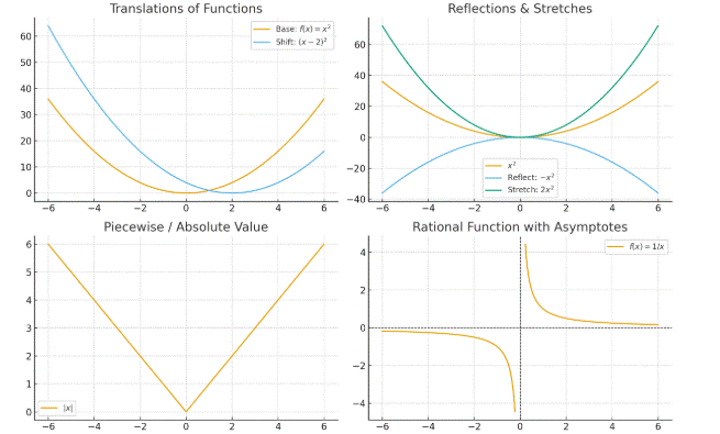
Transformations alter the shape or position of a function’s graph. They include translations (shifts), reflections, stretches, and compressions. Transformations allow us to study the effect of parameters on functions.

• Vertical translation: f(x)+k → shifts graph up/down.
• Horizontal translation: f(x−h) → shifts graph left/right.
• Reflection: −f(x) (across x-axis), f(−x) (across y-axis).
• Stretch/compression: af(x) (vertical), f(bx) (horizontal).

Example:
If f(x)=x², then:

• f(x)+3=x²+3 → parabola shifted up 3.
• f(x−2) =(x−2)² → parabola shifted right 2.
• −f(x)=−x² → reflection across x-axis.
• 2f(x)=2x² → vertical stretch.

2. Composite Transformations

Definition:
When multiple transformations occur, order matters. Generally, transformations are applied inside parentheses first (horizontal), then outside (vertical).

Example:
Take f(x)=x². Build g(x)=−2(x−3)²+4.

• (x−3)² → shift right by 3.
• −2(x−3)² → reflection + vertical stretch by 2.
• −2(x−3)²+4 → shift up 4.
  The final graph is a parabola opening down, vertex at (3,4).

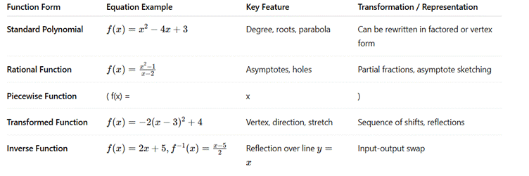
3. Equivalent Representations of Polynomial & Rational Expressions

Definition:
A single function can have multiple algebraic forms. These equivalent representations reveal different features.

• Polynomial forms: Standard form axⁿ+…+c, factored form (roots), vertex form (quadratics).
• Rational functions: Factorization vs. partial fractions.

Example:
Polynomial: f(x)=x²−5x+6=(x−2) (x−3). Factored form directly shows roots at 2 and 3.

Rational:

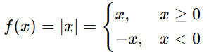
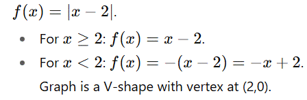
4. Piecewise and Absolute Value Transformations

Definition:
Piecewise functions use different rules for different domains. Absolute value creates a V-shape graph and can be viewed as piecewise:
 

Example:

5. Model Selection in Real-World Scenarios

Definition:
Choosing the right model depends on context. Polynomials often model smooth growth/decline, rational capture restrictions/asymptotes, exponentials handle rapid growth/decay.

Example:

• Population growth → exponential model.
• Projectile motion → quadratic model.
• Rate of chemical reaction (Michaelis-Menten equation) → rational model.

If data shows diminishing returns (growth slows over time), a rational model may fit better than a polynomial.

6. Assumption Articulation in Modeling

Definition:
When building mathematical models, assumptions must be stated clearly (e.g., ignoring friction, constant rate, continuous growth). They simplify real-world systems for analysis.

Example:
Modeling a car’s braking distance:

• Assume uniform deceleration.
• Model: s=v²/2a​, where v = velocity, a = deceleration.
  This assumption ignores factors like road conditions or driver reaction time.

7. Function Construction from Conditions

Definition:
Sometimes models are built directly from given conditions (e.g., intercepts, slopes, asymptotes).

Example:
“Find a quadratic with vertex (2,3) and passing through (0, -1).”

• General vertex form: f(x)=a(x−2)²+3.
• Plug in (0, -1): −1=a (0−2)²+3⇒−1=4a+3⇒a=−1.
• Final: f(x)=−(x−2)²+3.

8. Inverse Functions and Their Representations

Definition:
An inverse swaps input and output. Graphically, the inverse is the reflection across y=x. Algebraically, solve for x in terms of y.

Example:
f(x)=2x+5.

• Replace f(x) with y: y=2x+5.
• Swap: x=2y+5.
• Solve: y=x−5/2.
  Thus, f^-1(x)=x−5/2​.

9. Graphical vs Algebraic Models

Definition:
Functions can be represented in multiple ways:

• Graphical: visual trends, symmetry, asymptotes.
• Algebraic: precise symbolic manipulation.
• Tabular: discrete data values.

Example:
Function f(x)=1/x​.

• Graph: Hyperbola with vertical/horizontal asymptotes.
• Algebraic: Compact equation form.
• Table: f (1) =1, f (2) =0.5, f (10) =0.1.

10. Applications of Models in Prediction

Definition:
Functions are used to forecast outcomes in real-world contexts. Validity depends on assumptions and data range.

Example:
Finance: Compound interest

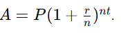
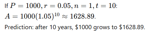
Table: Forms & Transformations of Functions

Transformations and Representations of Functions

Example: –

A freshwater-ecology team wants a model for the size of a fish population F(t) (number of fish) in a pond, where t is months since monitoring began (t≥0). Observed behaviour and requirements:

• Initial population at t=0 is 50 fish.
• Early growth is accelerated (approx. quadratic trend) because of abundant food.
• Long-term carrying capacity (maximum sustainable population) is about 300 fish.
• Management will shift the growth curve (slight delay then faster early growth) — i.e., apply transformations to the base polynomial model.
• There is a seasonal fluctuation (±8%) due to temperature cycles.
• After month 10 a regulated harvesting policy reduces population linearly with time.
• The team wants to know when (month t) the population will first reach 200 fish (before harvesting starts).
• State assumptions used to build the model.

Solution: –

1) Model construction from conditions

We choose a base polynomial to capture early accelerated growth (quadratic is simple yet flexible). Let

Why these coefficients?

• P (0) =50 (initial condition satisfied).
• Quadratic coefficient 5>0 gives accelerating growth in early months.
• Linear term 20t adds steady early growth.

(We could have used vertex form and solved for coefficients from conditions; here coefficients were chosen to match the qualitative requirements and P (0) =50.)

2) Function transformations — basics & composite transformations

Management wants the growth curve delayed slightly (shift right by 0.5 months), stretched vertically by 1.2 (early growth stronger after interventions), and offset downward by 10 to reflect immediate mortality from handling.

We apply these sequential transformations to the base polynomial:

• Horizontal shift right by 0.5: P(t−0.5).
• Vertical stretch by 1.2: 1.2 P(t−0.5).
• Vertical translation down by 10: Q(t)=1.2 P(t−0.5) −10.

Compute P(t−0.5) first:

So, Q(t) is the transformed polynomial representing potential population before seasonal effects and saturation.

3) Equivalent representations

We now have multiple forms:

• Base polynomial: P(t)=5t²+20t+50.
• Transformed polynomial (expanded): Q(t)=6t²+18t+39.5.
• Factored / vertex forms could be computed if desired (but expanded form is convenient for algebraic manipulation required later).

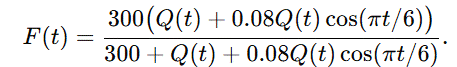
4) Apply seasonal multiplicative factor

Seasonal fluctuation is multiplicative: fish reproduction efficiency oscillates ±8% annually with period 12 months. A simple periodic factor:

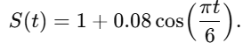
Combined (before saturation):

So, R(t) models the environmentally adjusted potential population (no carrying capacity yet).

5) Introduce carrying capacity — rational saturation model

To reflect a carrying capacity K=300 (long-term maximum), we use a standard saturating rational representation that maps an unbounded input into a value below K:

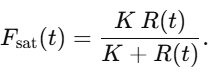
This rational form has the property that as this captures diminishing returns and saturation. (This choice is a modeling decision — a logistic function could be used instead; we justify the rational choice in the assumptions section.)

So, for months before harvesting:

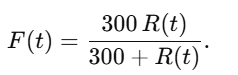
This is a rational function whose numerator and denominator are polynomials (after expanding R(t), so it fits our unit’s rational representation topics.

6) Piecewise behavior, representation, and prediction

Final numerical result

• The model (with chosen parameters) predicts the population reaches 200 fish at approximately t≈8.38 months (first time, prior to harvesting).

 Five Conclusive Points

1. Transformations unify function behavior – Shifts, reflections, and stretches are essential tools to adapt base functions into real-world patterns.
2. Equivalent forms enhance flexibility – Standard, factored, vertex, piecewise, or rational representations each reveal unique insights for problem solving.
3. Modeling requires assumptions – Every real-world application (finance, biology, physics) demands clearly stated simplifications for accurate function construction.
4. Multiple representations aid interpretation – Graphs, equations, and tables complement one another, providing a complete picture of function dynamics.
5. Applications validate models – The strength of any function model lies in its ability to predict trends, match observed data, and adjust to constraints.