Building And Reversing Functions: Composition & Inverses

Unit: Exponential & Logarithmic Functions

Chapter: Building and Reversing Functions: Composition & Inverses

Reference: – Introduction to Function Composition, Domain & Range in Composition, Properties of Composition, Exponential Functions in Composition, Logarithmic Functions in Composition, Inverse of a Function (Definition), Finding Inverses of Exponentials, Finding Inverses of Logarithms, Graphical Symmetry in Inverses, Applications of Composition & Inverses

After studying this chapter, you should be able to:

• Introduction to Function Composition & Domain & Range in Composition
• Properties of Composition & Exponential Functions in Composition
• Finding Inverses of Exponentials & Finding Inverses of Logarithms
• Applications of Composition & Inverses

1. — Introduction to Function Composition

Definition and theory: Composition is the operation of applying one function to the result of another. If one function is named f and another is named g, then the composition f of g is the function that takes an input, feeds it to g, and then feeds the output of g to f. Composition is a way to build complex transformations from simpler pieces and is central to function building, modeling layered processes, and expressing nested relationships. Composition is sensitive to order: applying f after g is generally different from applying g after f.

Example: Consider an outer effect that scales any input multiplicatively and an inner effect that translates the input. The composed mapping first translates the original variable and then scales the translated value. As a modeling thought experiment, this can represent a physical process where a preparatory change occurs before a proportional amplification.

2. — Domain and Range in Composition

Definition and theory: When composing two functions, the domain of the composition is constrained by both functions. Formally, the composition f of g is defined only for inputs that belong to the domain of g whose images under g belong to the domain of f. Thus, composition can introduce implicit restrictions that are not visible when each function is considered separately. Understanding these restrictions is crucial for valid algebraic manipulation and for interpreting models correctly.

Example: Suppose g maps inputs to strictly positive outputs, and f is defined only for positive inputs. Then the composition f of g is defined on all inputs where g is defined; however, if g sometimes produces nonpositive values the composition would be undefined there. In modeling terms, an instrument that outputs concentrations only above a threshold can be composed with a response function that requires above threshold values, enforcing a domain compatibility condition.

3. — Properties of Composition

Definition and theory: Composition is associative: composing three functions in a chain can be grouped in any way without changing the resulting mapping. Composition is generally noncommutative: swapping the order of two functions typically produces a different mapping. The identity function acts as a neutral element under composition: composing any function with the identity on the appropriate domain leaves the function unchanged. These properties are used to manipulate expressions, to simplify nested maps, and to construct inverses via composition with the identity.

Example: Given three transformations representing, respectively, an initial calibration, a sensor response, and a postprocessing normalization, associativity guarantees that grouping the first two then the third yields the same overall transformation as grouping the first with the composition of the last two. Noncommutativity warns that if normalization is applied before sensor response the result differs from normalizing after sensing.

4. — Exponential Functions in Composition

Definition and theory: Exponential functions appear naturally in composition when an exponential mapping is applied after, or before, another transformation. Composing a linear shift or affine transformation into the exponent shifts or rescales the growth pattern, while composing an exponential into another function can model multiplicative effects layered with other transformations. Because exponentials amplify input differences multiplicatively, they can dramatically change the sensitivity and long-term behavior of composed systems.

Example: Compose an exponential mapping with a time shift: first shift time by a delay operator, then apply an exponential growth mapping. This model delayed onset of multiplicative growth in a system where some preparatory stage must occur before exponential amplification begins. Alternatively, composing an exponential after a saturation mapping models growth that is capped before being amplified.

5. — Logarithmic Functions in Composition

Definition and theory: Logarithms are the inverse operations to exponentials and thus appear naturally when reversing exponential compositions or when composing with functions that require compression of large ranges into manageable scales. Composing a logarithm after a multiplicative process linearizes multiplicative relationships, making them easier to analyse and handle. Conversely, composing a logarithm before another nonlinear map can reduce sensitivity to scale and stabilize inputs.

Example: Imagine a measurement instrument whose output grows multiplicatively with the physical quantity of interest; composing a logarithm after the instrument yields a mapping on which additive noise models are more appropriate. This composition is used in many scientific models where multiplicative effects are linearized for regression or visualization.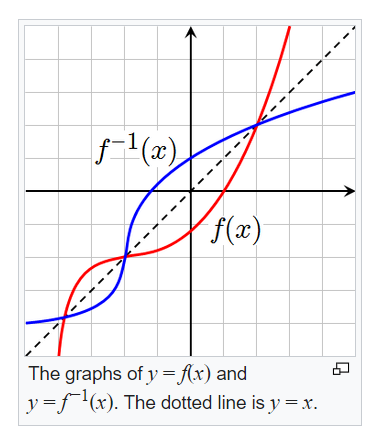

6. — Inverse of a Function (Definition and Existence Conditions)

Definition and theory: An inverse function undoes the effect of a function: if f maps an input to an output, then its inverse maps that output back to the original input. For a function to possess a global inverse on a given domain its mapping must be one to one on that domain so that each output corresponds to a unique input. When these conditions hold, composition of the function with its inverse yields the identity transformation in either direction. Inverse functions allow solving equations of the form f of x equals given value by applying the inverse to the given value.

Example: A strictly monotone increasing growth mapping on a suitable domain has an inverse that returns the original initiating magnitude when applied to the observed magnitude. In modeling, this allows reconstructing the initiating condition from an observed outcome by applying the inverse mapping.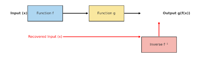

7. — Finding Inverses of Exponentials

Definition and theory: The inverse of an exponential mapping is a logarithmic mapping. To find the inverse in symbolic terms, one replaces the dependent variable with a placeholder, swaps dependent and independent variables, and then algebraically isolates the new dependent variable using the logarithm. Exponential inverses convert multiplicative, rapidly changing scales into additive, slowly varying scales. Care must be taken about domains: exponentials with positive base map into strictly positive outputs; consequently, logarithmic inverses are defined on positive values only.

Example: Given a mapping that raises a base to the power of a translated input, finding the inverse requires unwinding the translation and then taking the logarithm base the same as the original base. This inverse mapping returns the translated input from the observed exponential output, provided the observed output lies within the allowed positive range.

8. — Finding Inverses of Logarithms

Definition and theory: The inverse of a logarithm is an exponential mapping. Finding the inverse algebraically means swapping the roles of input and output and then raising the chosen base to the power of the new dependent variable. Logarithms compress multiplicative relationships; their inverses re-expand compressed values. Domain considerations again apply: the logarithm’s domain restricts its inverse and determines the valid inputs for the exponential that reconstructs original scales.

Example: If a function reports the logarithm of a physical quantity with respect to a chosen base, then the inverse mapping recovers the original quantity by exponentiation with that base. This procedure restores multiplicative scale from additive logged values and is fundamental in reversing linearized models.

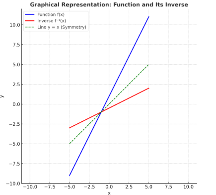
9. — Graphical Symmetry in Inverses

Definition and theory: Graphically, an inverse relationship corresponds to reflection across the diagonal line where the independent variable equals the dependent variable. This reflection property provides a visual test for invertibility on a region: if the original graph intersects any horizontal line at most once (horizontal line test), then the reflected graph will also be a well-defined function. The visual symmetry helps students and practitioners check for inverses and understand the mapping between inputs and outputs.

Example: Plot a mapping that steadily rises without turning back. Reflect that curve across the diagonal and observe that the reflected curve is also a single-valued mapping. This geometric reflection gives an immediate picture of how the inverse restores inputs from outputs.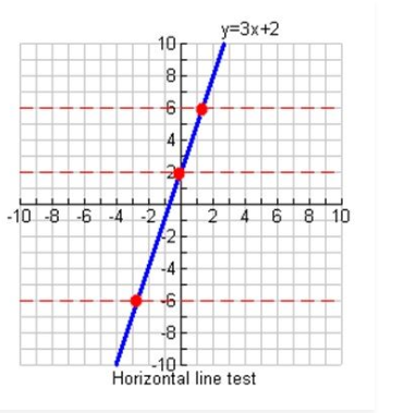

10. — Applications of Composition and Inverses

Definition and theory: Composition and inverses are central to modeling layered processes, solving for initiating conditions, transforming data scales, and building complex maps from simpler building blocks. Composition models sequential stages of a system; inverses permit recovery and decision making based on observed outcomes. In practice, these tools appear across disciplines: in finance for compounding and discounting, in physics for forward and inverse scattering problems, in biology for transforming growth measurements, and in data science for preprocessing pipelines and interpretation. Thoughtful use of composition and inversion requires clarity about domains, continuity, monotonicity, and units.

Example: A modeler composes a measurement apparatus mapping with a calibration mapping and then with a postprocessing normalization. To retrieve the original physical quantity from a processed reading, the modeler composes the inverses in the reverse order. Doing so reconstructs the initiating physical magnitude while revealing where measurement sensitivity or domain restrictions matter.

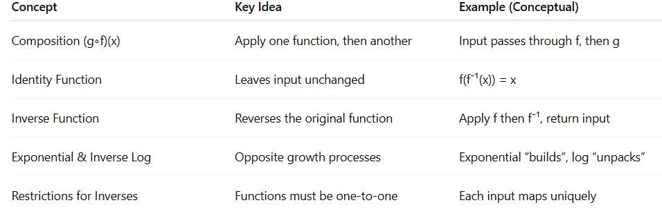
COMPARISON TABLE

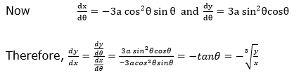
Example: – Find dydx, if x23+y23=a23

Solution: Let x = a cos³ θ , y = a sin³ θ

 x23+y23=(a cos3θ)23  + (a sin3θ)23  

 a23cos2θ+sin2θ=a23

Hence, x = a cos³θ , y = a sin³ θ  is parametric equation of x23+y23=a23  

Example: Find dydx  for y = e^{sin t} and x = 3t³.

Solution: y = e^{sin t}

dydt  = e^{sin t} (cos t)

x = 3t³

dxdt  = 9t²

dydx=dydtdxdt=esintcost9t2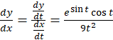  

Five Conclusive Points

1. Composition reveals complexity – Functions can be layered (e.g., g(f(x)), allowing more intricate models and transformations.
2. Inverses restore original input – Applying an inverse function reverses the effect of the original, ensuring reversibility.
3. Symmetry is key – Graphs of functions and their inverses mirror each other across the line y=x, giving a powerful geometric interpretation.
4. Restrictions matter – Not all functions have inverses; domain and range adjustments are essential to maintain one-to-one behavior.
5. Applications connect theory to reality – From encryption and decryption in computer science to logarithmic-exponential relationships in mathematics, composition and inverses are foundational.